TASC 2026.05 The AutoTune Filter█ OVERVIEW
This script implements the AutoTune Filter described by John F. Ehlers in the article "A Rolling Autocorrelation Function" from the May 2026 edition of the TASC Traders' Tips . The script analyzes rolling autocorrelation in filtered price data to calculate a band-pass filter that dynamically adjusts to apparent dominant cycles.
█ CONCEPTS
Autocorrelation function (ACF)
Autocorrelation measures the correlation of a time series with a lagged version of itself. The autocorrelation function (ACF) evaluates autocorrelation across a range of lags to gauge the extent to which values in a series vary jointly with previous values at different offsets.
The ACF can help traders identify patterns and trends in stochastic market data, characterize long-range dependence in a series, and more. In his article, Ehlers explains how the ACF can serve as a "bridge" between analysis in the time and frequency domains for identifying dominant cycles in market data.
Ehlers notes that at low lags, such as one bar, the autocorrelation in price data tends to be very high because prices don't often change dramatically from one bar to the next. As the lag increases, autocorrelation often decreases, reaching near zero for offsets at which the latest prices do not show a clear relationship with past prices.
However, he also observed that at specific lags, anticorrelation (negative correlation) can emerge, where the current values in the series move in one direction while past values move in the opposite direction. Based on this observation, he suggests that a lag with strong anticorrelation can indicate a significant cycle in the market data, where the cycle length is twice that of the analyzed lag.
To understand why this behavior can indicate significant cycles, consider a sine wave that completes a full oscillation every 20 bars. If the series is currently moving up, it will then move down 10 bars later, and then complete the cycle by moving up again 10 bars after that. The ACF of that sine wave returns a value of -1 for a lag of 10 bars, but not for other lower lags or higher lags up to 20.
In other words, a pure sine wave with a given period has perfect anticorrelation with a delayed version of itself that is offset by half of that period.
While market data does not typically behave like a pure sine wave, the same underlying principle applies: if the current prices exhibit a strong anticorrelation with previous prices at a given offset, a dominant cycle with a length of twice that offset is likely present in the current data.
AutoTune Filter
Ehlers proposes that traders can use the dominant cycle obtained via autocorrelation to set the critical period of a filter. Tuning a filter to respond most strongly to the measured cycle may promote more consistency in time alignment and help reduce destructive phase shifts.
He demonstrates one such implementation with his AutoTune Filter, an adaptive band-pass filter whose center period dynamically increments toward the dominant cycle calculated from an ACF over a given window.
The steps to calculate the AutoTune Filter are as follows:
Apply a two-pole high-pass filter to the series to reduce the effect of low-frequency (long-period) cycles on the autocorrelation calculation. The filtered series emphasizes cycles with lengths up to the specified cutoff period, and attenuates all others.
Compute the rolling ACF of the filtered data across the same window length as the filter's cutoff period.
Check the autocorrelation for each lag period, and identify the smallest lag with the lowest autocorrelation value. Multiply that lag by two to obtain the dominant cycle for the analyzed window.
If the difference between the current and previous dominant cycle is greater than two, limit the result for the current bar to two greater or less than the previous cycle's value to prevent large, sudden shifts in the filter's center period.
Finally, compute a band-pass filter using the value from step 4 as the center period.
█ USAGE
This indicator includes four display modes to visualize the AutoTune Filter's calculations:
"High-pass filter" : Plots the high-pass filtered data that the script analyzes for autocorrelation calculations.
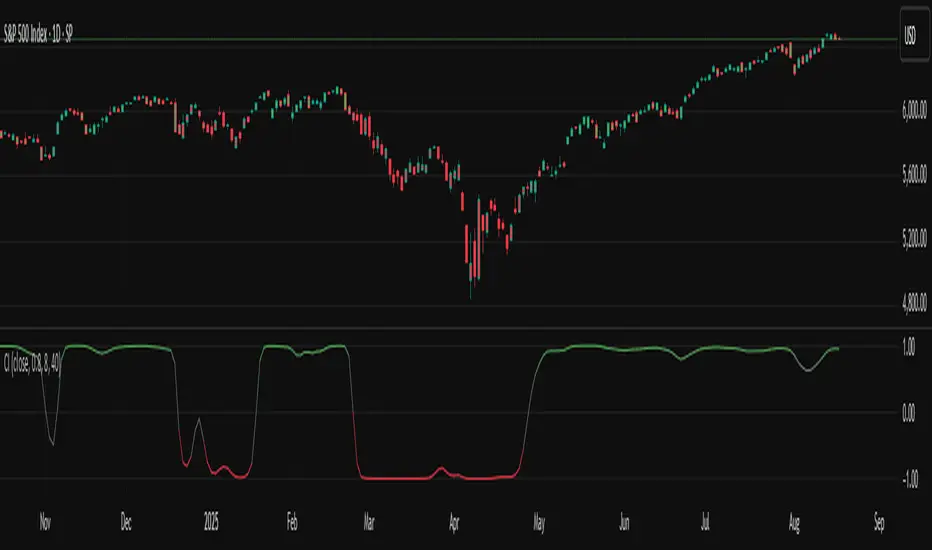
"Min. correlation" : Plots the lowest autocorrelation value calculated for the filtered series over the analyzed window.
"Dominant cycle" : Plots the dominant cycle value that the final filter uses for its center period.
"Tuned band-pass filter" (default): Plots the final band-pass filtered result, i.e., the AutoTune filter.
Ehlers suggests that traders can identify peaks and valleys in prices for potential mean reversion signals by analyzing the rate of change in the tuned band-pass filter. If the rate of change is zero, the current price might be near a local high if the filter's value is positive, or near a local low if the value is negative.
Users can analyze the additional outputs to gain further insight into the filter's behaviors, and they can pass these plotted values to other scripts via source inputs for easy use in other custom calculations.
█ INPUTS
The indicator includes the following inputs in the "Settings/Inputs" tab:
Source: The series of values to process.
Window: The window length of the ACF calculation, and the cutoff period of the high-pass filter. The maximum possible dominant cycle length is two times this value.
Output: One of the four display modes ("High-pass filter", "Min. correlation", "Dominant cycle", or "Tuned band-pass filter").
Ehlers
Market Volatility Momentum & Trend Filter Pro @MaxMaserati 3.0
Market Volatility Momentum & Trend Filter Pro (MVM 3.0)
The Market Volatility Momentum & Trend Filter Pro (MVM 3.0) is an institutional-grade technical analysis suite built upon the foundations of Digital Signal Processing (DSP), Auction Market Theory, and Order Flow Delta. This version integrates advanced filtering techniques to distinguish between high-conviction trend expansions and low-conviction liquidity traps.
1. Digital Signal Processing & Ehlers Integration
A core differentiator of MVM 3.0 is the integration of advanced DSP filters inspired by the pioneering work of John F. Ehlers. Rather than relying on traditional moving averages—which suffer from significant lag and spectral leakage—this script employs high-order filters to isolate the "signal" from market "noise."
SuperSmoother Filter:Based on Ehlers' research, the SuperSmoother is a two-pole Butterworth filter designed to provide superior noise reduction with minimal lag. It effectively removes aliasing and high-frequency cycles that often trigger false signals in standard indicators.
Two-Pole Momentum Filter:This component utilizes a sophisticated damping coefficient to create a smooth, responsive trend line. The mathematical construction follows the logic of a second-order system:
f1 = f1 + alpha * (source - f1 )
f2 = f2 + beta * (f1 - f2 )
Market Cycle Sine-Wave: Using Ehlers-inspired cycle extraction techniques, the script identifies the dominant market rhythm, allowing traders to see the "phase" of the current move (Accumulation, Expansion, or Exhaustion).
2. Structural Architecture: The HTF Fused Midpoint
The primary directional filter of the system is the HTF Fused Midpoint. This dynamic line acts as a structural equilibrium point by calculating data from a higher timeframe (HTF) relative to the current chart.
Auto-HTF Selection: The system automatically identifies the most relevant higher timeframe (e.g., pulling 1H data for a 15m chart) to provide a macro context for micro-level entries.
Midpoint Calculation: It identifies the 14-period high and low of the HTF and plots the 50% retracement level, which serves as a binary filter for trend bias.
3. Momentum Pivot: Volume Profile & POC
To provide institutional context, MVM 3.0 integrates a rolling Volume Profile engine based on Auction Market Theory.
Point of Control (POC): This is the "Momentum Pivot"—the price level where the highest volume was transacted during the specified lookback period.
Value Area (VAH/VAL): The script dynamically calculates the range where 70% of the volume occurred.
Premium Zone: Above VAH (Potential exhaustion or breakout).
Discount Zone: Below VAL (Potential accumulation or breakdown).
Fair Value: Inside the Value Area (Mean reversion or balance environment).
4. Intelligent Candle Logic & Order Flow
The decision engine of MVM 3.0 processes real-time Exchange Footprint (Delta) data to validate price movement.
Trend Start (PO4 Equivalent): Triggered when a breakout candle crosses the HTF Midpoint, confirmed by the Ehlers Cycle Filter.
Breakout / Breakdown: Confirmed when price breaches volatility bands accompanied by Strong Delta (aggressive market participation).
The Trap Candle: A critical risk-management feature. It triggers when an expansion candle occurs while the Market Cycle is at an exhaustion threshold (calculated via Mean Absolute Deviation) and the Delta is weak. This identifies "Liquidity Sweeps" where aggressive participants are failing to sustain momentum.
5. Quantitative Dashboard
The integrated dashboard provides a real-time summary of the technical environment:
Trend State: Classifies the current phase as Discovery, Breakout, or Neutral.
Zone Analysis: Monitors price location relative to the Volume Profile Value Area.
Market Cycle: Alerts to "Extreme" conditions where the current move may be overextended.
Bar Delta: Displays the percentage of aggressive buying versus selling in the current candle.
Credits
Special credit is given to John F. Ehlers for his extensive research into Digital Signal Processing for traders. The implementation of the SuperSmoother and Two-Pole Filters within this script is derived from his mathematical models for noise reduction and cycle analysis in financial markets.
Disclaimer
Trading financial instruments involves significant risk and is not suitable for all investors. The Market Volatility Momentum & Trend Filter Pro (MVM 3.0) is a technical analysis tool provided for educational and informational purposes only. It does not constitute investment advice, financial advice, or a recommendation to trade. Performance seen in historical data is no guarantee of future results. The user assumes full responsibility for any trading decisions and should implement a comprehensive risk management strategy. Use of Footprint/Delta features requires a TradingView plan and data feed that supports intraday tick data.
Pine Script® indicator
MESA Adaptive Cycle Engine [MarkitTick]💡 The MESA Adaptive Cycle Engine is an advanced, dynamic trend-following overlay designed to adapt to market volatility and cyclical phases. Unlike traditional moving averages that suffer from significant lag during range-bound periods, this tool leverages digital signal processing to stay aligned with the market's dominant cycle. It features an integrated webhook automation system and a real-time risk management dashboard.
✨ Originality and Utility
Standard exponential or simple moving averages rely on fixed lookback periods, making them inherently flawed when market conditions shift from trending to cycling. This indicator utilizes the MESA (Maximum Entropy Spectral Analysis) Adaptive Moving Average (MAMA) and Following Adaptive Moving Average (FAMA) concepts. By measuring the phase rate of change via a Hilbert Transform, the moving averages mathematically adapt their alpha speeds. Furthermore, this script is uniquely engineered for modern automated trading, featuring a self-cleaning dashboard and dynamically constructed JSON payloads for external execution engines.
🔬 Methodology and Concepts
● The Hilbert Transform
At its core, the script applies a Hilbert Transform to the price source (defaulting to hl2) to extract the real and imaginary components of the market cycle.
● Phase and Period Calculation
By calculating the arctangent of the quadrature and in-phase components, it determines the current phase and dominant cycle period.
● Adaptive Alpha
The phase's rate of change dictates the alpha variable. In trending markets, the phase changes slowly, allowing the alpha to remain near the Fast Limit. In choppy markets, the phase changes rapidly, dropping the alpha toward the Slow Limit to prevent whipsaws.
● Risk Engine
The script establishes automated Stop Loss and Take Profit levels based on an ATR multiplier, updating dynamically upon regime shifts.
🎨 Visual Guide
● MAMA and FAMA Lines
The indicator plots two primary lines: the MAMA line (default Green) and the FAMA line (default Red).
● Regime Fill
The space between MAMA and FAMA is filled with a semi-transparent Bullish color when MAMA is above FAMA, and a Bearish color when MAMA is below FAMA.
● Entry Signals
A small upward triangle is plotted below the bar upon a Golden Cross (Buy Signal), and a downward triangle is plotted above the bar upon a Death Cross (Sell Signal).
● Analytics Dashboard
A table in the bottom-right corner displays the current Market Regime, Phase Volatility (ATR), and the active JSON Payload status.
📖 How to Use
Wait for a confirmed crossover. A Golden Cross (MAMA crossing above FAMA) initiates a Bullish regime, while a Death Cross initiates a Bearish regime.
Use the Regime Fill to hold positions; stay in a long position as long as the fill remains bullish.
Monitor the Dashboard for real-time ATR values to assist with manual trailing stops, or rely on the automated Risk Manager's calculated Take Profit (2x ATR) and Stop Loss (1x ATR).
Non-standard charts (like Heikin Ashi or Renko) will trigger a runtime warning, as cycle measurements rely on standard time-based OHLC data.
⚙️ Inputs and Settings
● MESA DSP Parameters
Price Source: Determines the input data (default hl2).
Fast Limit: The maximum alpha speed, usually set to 0.5.
Slow Limit: The minimum alpha speed, usually set to 0.05.
● Automation & JSON Payload
ATR Multiplier: Controls the width of the Stop Loss and Take Profit levels.
Webhook Action (Long/Short): Defines the string action injected into the outgoing JSON payload.
🔍 Deconstruction of the Underlying Scientific and Academic Framework
The indicator is deeply rooted in digital signal processing (DSP), specifically pioneered for trading by John Ehlers. The framework models market data as a complex waveform. By passing the data through a 4-bar WMA smoother and then applying a Hilbert Transform, the algorithm isolates the in-phase (I) and quadrature (Q) components. This orthogonal relationship allows the script to map the market's analytic signal onto a complex plane, solving for the instantaneous phase angle. The fundamental academic breakthrough here is using the derivative of this phase (the rate of phase change) to govern the exponential smoothing constant (alpha) of the moving average. This ensures the filter's bandwidth dynamically conforms to the signal's spectral density, offering high-fidelity smoothing without the commensurate group delay found in static linear filters.
⚠️ Disclaimer
All provided scripts and indicators are strictly for educational exploration and must not be interpreted as financial advice or a recommendation to execute trades. I expressly disclaim all liability for any financial losses or damages that may result, directly or indirectly, from the reliance on or application of these tools. Market participation carries inherent risk where past performance never guarantees future returns, leaving all investment decisions and due diligence solely at your own discretion.
Pine Script® indicator
TASC 2026.04 A Synthetic Oscillator█ Overview
This script implements a Synthetic Oscillator as presented by John F. Ehlers in the April 2026 TASC Traders' Tips article "Avoiding Whipsaw Trades". The indicator aims to provide a smooth, low-lag oscillator for timely trading signals by dynamically mapping a sine wave to price data.
█ CONCEPTS
"Whipsaw" trades are a common issue in algorithmic trading. They occur when the market quickly moves against a position, causing the trader/trading system to reverse their position at a loss, and then the market reverses again and continues in the original direction. Such trades occur because the trading system is attempting to react quickly to market moves instead of focusing on broader market cycles.
A typical solution for reducing whipsaw trades is to apply linear filters to smooth the data and emphasize specific cycles. However, linear filters cannot have both a smooth response and a low computational lag. Therefore, strategy designs utilizing linear filters require a tradeoff between smoothness and lag.
Ehlers proposes a nonlinear indicator as a solution to bridge the gap and achieve a smooth, timely response while reducing whipsaw trades.
The Synthetic oscillator adapts to market conditions by calculating a dynamic sine wave from the estimated instantaneous dominant cycle over a range of periods.
The process to calculate the indicator is as follows:
Smooth the price data with a 12-bar Hann Window filter to reduce high-frequency noise, which can affect dominant cycle estimates.
Band-pass filter the windowed data with a two-pole high-pass filter and a SuperSmoother filter to focus on the range of cycles between a specified lower bound and upper bound, and normalize the result using the filter's 100-bar root mean square (RMS).
Calculate the one-bar rate of change (ROC) in the oscillator from step 2, and normalize the ROC using its 100-bar RMS.
Estimate the instantaneous dominant cycle from the oscillators in steps 2 and 3 by treating the series as a complex waveform , where the first oscillator represents the waveform's band-limited "real" component ("I"), and the second represents the band-limited "imaginary" component ("Q").
Cumulatively sum the reciprocal of the dominant cycle (i.e., the dominant frequency ) to obtain the phase angle of the sine wave.
To reduce cumulative errors and lag in the phase angle calculation, compute a secondary band-bass filter from a high-pass filter and the UltimateSmoother, and reset the angle to 0 or 180 degrees when that filter crosses above or below 0.
Calculate the Synthetic Oscillator as the sine of the final phase angle.
█ USAGE
This indicator displays the Synthetic Oscillator and a horizontal zero line in a separate pane. Users can analyze the crossings between the oscillator value and 0, or the behavior of the oscillator as it reaches 1 or -1, to derive potential timely trading signals.
Ehlers notes in the article that the peaks and valleys of the Synthetic Oscillator can provide signals a little too early, depending on the settings and context. Therefore, he recommends applying another smoother to the oscillator, such as a Hann Window filter with an optimizable length, to adjust timing as necessary.
█ INPUTS
This indicator uses multiple hardcoded parameters based on the implementation in Ehlers' article. However, users can customize the source series and the upper and lower bounds of the calculations:
Source Series: The series of values to process.
Lower Bound: The smallest cycle in the passband of the filters, and the lower limit of the dominant cycle estimate.
Upper Bound: The largest cycle in the passband of the filters, and the upper limit of the dominant cycle estimate.
Ehlers Decycler (DECYCLER)The Ehlers Decycler extracts the trend component from a price series by subtracting a 2-pole Butterworth high-pass filter from the source. Cycles shorter than the cutoff period are removed; everything longer passes through with near-zero phase lag. The result is a trend overlay that tracks price more closely than a comparable EMA during trends, with no smoothing window, no lag-versus-smoothness tradeoff, and exactly one parameter.
HISTORICAL CONTEXT
John Ehlers introduced the Decycler in "Decyclers" ( Technical Analysis of Stocks & Commodities , September 2015), alongside its oscillator companion DECO. The underlying 2-pole Butterworth high-pass filter had appeared in Ehlers' earlier work ( Cybernetic Analysis for Stocks and Futures , 2004), primarily for cycle measurement. The Decycler simply inverts the question: instead of isolating cycles, subtract them. What remains is trend.
The approach sidesteps the fundamental tension in trend-following design. Moving averages introduce lag proportional to their smoothing window. Adaptive averages reduce lag but add parameters and complexity. The Decycler reframes the problem as a frequency-domain operation: define a cutoff period, remove everything above it, keep everything below. The phase response of the complementary filter preserves the phase of passed frequencies — trend components below the cutoff experience near-zero lag by construction, not by approximation.
HOW IT WORKS
Stage 1 — 2-pole Butterworth high-pass filter
A single coefficient α is derived from the cutoff period P using the Butterworth −3 dB design point (the 0.707 = 1/√2 factor places the half-power point at exactly period P):
ω = 0.707 × 2π / P
α = (cos(ω) + sin(ω) − 1) / cos(ω)
Three recurrence coefficients are computed once at construction from α:
a₁ = (1 − α/2)² ← input gain
b₁ = 2(1 − α) ← first feedback
c₁ = −(1 − α)² ← second feedback
The HP recurrence runs each bar:
HP = a₁ × (x − 2x + x ) + b₁ × HP + c₁ × HP
The second-difference term (x − 2x + x ) is a discrete second derivative — it rejects DC and linear trends while passing oscillatory content, which the HP feedback then sharpens into a proper bandpass edge.
Stage 2 — Complementary subtraction
The Decycler is one line:
Decycler = x − HP
This guarantees that Decycler + HP = price at every bar. No signal energy is created or destroyed. The trend and cycle components sum exactly to the original series.
Frequency response
- Periods longer than the cutoff: unity gain, near-zero phase shift.
- Periods shorter than the cutoff: attenuated at −12 dB/octave (2-pole rolloff).
- At exactly period P: −3 dB (≈29% amplitude reduction).
INPUTS & PARAMETERS
- Source — Input series. Default: close.
- Period — Cutoff period in bars. Cycles shorter than this are removed. Default: 60.
Period selection
- 20–30: Responsive trend line, tracks swings. Short-term trading on daily bars.
- 40–80: Balanced separation. Default of 60 works well for daily timeframes.
- 100–200: Heavy smoothing, reveals major trend direction only. Position trading and regime detection.
Ensure the dataset has at least 2 × period bars for meaningful trend extraction. On a 100-bar chart, a period of 200 removes almost nothing — the cutoff falls below the Nyquist limit of the data.
HOW TO USE
Trend direction
- Price above Decycler → bullish. Price below → bearish.
- Slope of Decycler indicates trend momentum. Flattening slope → potential exhaustion or transition.
Trend vs. cycle regime
- Decycler hugging price closely → trending: the dominant cycle is shorter than the cutoff and is being removed, leaving clean trend.
- Decycler oscillating with small amplitude → ranging: price is spending time in both directions relative to the trend line.
Multi-period overlay
- Two Decycler instances at different periods (e.g., 30 and 120) reveal short-term and long-term trend simultaneously. Their relationship is interpretable in frequency terms — the gap between them is a specific cycle band.
Cycle complement
- The HP component (price − Decycler) isolates the cycle content. Plot it separately as a zero-mean oscillator to see what the Decycler is removing. If the cycle is large relative to trend, reduce position size.
This is not a moving average
- The Decycler does not compute a weighted sum of past prices. During strong trends it tracks price more closely than a same-period EMA. During ranging conditions it can exhibit small oscillations that a moving average would suppress. Factor this into signal logic.
LIMITATIONS
- Period too short: A cutoff of 10 on daily bars removes only cycles shorter than 10 days — nearly everything passes through and the Decycler approximates raw price. Meaningful separation requires the cutoff period to exceed the dominant cycle in the data.
- Not DECO: The Decycler is a lowpass trend overlay (price − HP). The Decycler Oscillator (DECO) is HP_long − HP_short — a bandpass oscillator that crosses zero. They share the same filter core but produce fundamentally different outputs. Using one where the other is needed produces incorrect results silently.
- Warmup: The HP recurrence requires two prior source values and two prior HP values. For the first two bars, HP = 0 and Decycler = raw price. IsHot = true after period bars; signals before that point are unreliable.
- IIR drift: Feedback terms accumulate floating-point error over very long series (> 10,000 bars). For typical trading horizons (< 5,000 bars), drift stays below 1e−10 and is inconsequential.
- No external validation baseline: TA-Lib, Skender, Tulip, and OoplesFinance do not implement the Ehlers Decycler. Validation is against the Pine reference implementation and internal streaming/batch/span consistency.
REFERENCES
- Ehlers, J. F. (2015). "Decyclers." Technical Analysis of Stocks & Commodities , September 2015.
Pine Script® indicator
EDCF: Ehlers Distance Coefficient FilterThe Ehlers Distance Coefficient Filter (EDCF) is a nonlinear adaptive FIR filter that computes its smoothing weights dynamically from the sum of squared price differences across the observation window. Recent bars that diverge most from the rest of the window receive the highest weight, making the filter faster than a comparable SMA in trending conditions while degenerating to a simple average when prices are flat.
HISTORICAL CONTEXT
John F. Ehlers introduced EDCF in "Nonlinear Ehlers Filters" ( Stocks & Commodities , V.19:4, 2001) and in the accompanying MESA Software paper. The core insight: instead of fixing weights by position (as EMA or WMA do) or by spectral design (as Ehlers' own Laguerre and MESA filters do), let the price data itself determine how much each bar contributes. Bars that are close in price to their neighbors get low weight; bars that represent breakouts or large moves get high weight. Ehlers specifically chose squared distances over Euclidean distances to amplify the response to large price changes.
HOW IT WORKS
For each bar, EDCF evaluates the last length bars and assigns each a coefficient based on its total squared distance from all other bars in the window.
Step 1 — Distance-squared coefficient
For each bar position i in the window, compute how different its price is from every other bar in the window:
Dist² = Σ (Price − Price )² k = 1 to length−1
A bar surrounded by similar prices gets a low coefficient. A bar at the edge of a sharp move gets a high one.
Step 2 — Normalized weighted average
The output is the weighted average of all bars, normalized by the total weight:
EDCF = Σ(Dist² × Price ) / Σ(Dist² )
Flat-price fallback
When all prices in the window are identical, all distance-squared coefficients are zero. The filter falls back to the current price — equivalent to SMA behavior with zero lag.
Why squared distances?
Ehlers explicitly chose Σ(diff²) over √(Σ(diff²)) to heighten filter response. Squaring amplifies the weight difference between trending and ranging bars, making the adaptive effect more pronounced.
INPUTS & PARAMETERS
- Source — Input series. Default: close.
- Length — Filter window length. Default: 15. Range: ≥ 2.
Larger length → smoother output, more lag, higher computational cost (O(length²) per bar).
Practical ceiling for real-time use: length ≤ 30. Above that, the nested loop becomes expensive on tick data.
HOW TO USE
Apply as a trend-following overlay on any instrument and timeframe.
Trend following
- In a trending market, EDCF weights the most-displaced bars heavily and tracks price more closely than a same-period EMA. Use it as a dynamic trailing reference.
- Price above EDCF → bullish bias. Price below → bearish bias.
Ranging detection
- When EDCF flattens and price oscillates tightly around it, the filter is approximating an SMA — a signal that the market has entered consolidation and trend-following signals should be discounted.
Breakout confirmation
- A sharp price extension that pulls EDCF steeply in one direction indicates the recent bars carry high distance-squared weight — confirmation that the move is statistically significant relative to the recent window, not just noise.
Asymmetric behavior awareness
- In a strong trend, EDCF behaves like a trailing stop: it follows closely in the direction of the trend but lags on reversals. Factor this into exit timing.
LIMITATIONS
- O(n²) complexity: Each bar requires a nested loop over the window. At length = 15 the cost is ~400 cycles/bar; at length = 30 it is ~1500 cycles/bar. Keep length ≤ 30 for real-time tick processing.
- Not an IIR filter: Despite being categorized as a filter, EDCF is a purely FIR structure — finite window, no feedback. It has no pole dynamics, unlike Ehlers' Laguerre or MESA SuperSmoother.
- Asymmetric lag: Response is faster in the direction of existing momentum and slower on reversals. This is a feature in trending regimes and a liability at turning points.
- No direct validation baseline: TA-Lib, Skender, and Tulip have no equivalent function. Validation is against the original Ehlers paper formulation and internal streaming/batch/span consistency.
- Warmup: Requires length bars before IsHot = true. Earlier outputs are provisional.
REFERENCES
- Ehlers, J. F. "Nonlinear Ehlers Filters." Stocks & Commodities , V.19:4, pp. 25–34, 2001.
- Ehlers, J. F. "Ehlers Filters." MESA Software technical paper.
Pine Script® indicator
Trend Sniper v2.5 [Jamallo](2025)
Intro
Trend Sniper v2.5 is built around a novel-unique core construction —
the Butterworth Stop : a ratcheting trailing stop anchored to a 2-Pole Butterworth Super Smoother and dynamically sized by Parkinson Volatility.
While each algorithm used is individually well-documented, this specific combination is rare and not found in standard indicator libraries — most Butterworth implementations are simply plotted as trend lines, not used as the structural anchor of a volatility-adaptive stop mechanism.
Break down:
2-Pole Butterworth Super Smoother (Core Trend Line) (smoothed price)
The backbone of the indicator is a 2-Pole Butterworth Super Smoother, a concept brought into trading by engineer and author John Ehlers, first published in his 2004 book Cybernetic Analysis for Stocks and Futures
In this indicator: The Butterworth filter runs on close with a user-defined period (default 20) and produces bw_trend — a clean, lag-minimized version of price. This smoothed value is not plotted directly. Instead, it acts as the anchor point for the trailing stop. The stop is placed at bw_trend ± stop_dist , meaning the stop hugs the filtered trend rather than raw price, making it far less susceptible to wick noise and erratic bars. Without this pre-filtering step, the trailing stop would oscillate erratically on volatile bars.
Parkinson Volatility (Sizes the Stop Distance)
"Developed by physicist Michael Parkinson in 1980, it estimates volatility using the natural logarithm of the high-to-low ratio each period, capturing intraday range rather than just close-to-close movement."
In this indicator: Parkinson Volatility is calculated over a rolling window (default 50 bars) and multiplied by stop_mult (default 1.2) to produce stop_dist . When markets are volatile, stop_dist expands and the stop gives price more room. When markets are quiet, it contracts and the stop tightens.
Butterworth Stop State Machine (The Main Line You Watch)
This is the primary plotted line, It's a classic ratcheting trailing stop built on top of outputs from steps 1 and 2.
In this indicator: The logic is a simple state machine with two modes — uptrend and downtrend. In an uptrend, the stop only moves up (never down), tracking at bw_trend − stop_dist . In a downtrend, it only moves down, tracking at bw_trend + stop_dist . When price closes on the wrong side of the stop, the state flips and the stop resets on the other side of the trend line. Because both the anchor bw_trend and the buffer stop_dist are noise-filtered and volatility-adjusted, the BW Stop flips far less often than a raw price-based trailing stop would, keeping you in trends longer.
Chande Momentum Oscillator + Deadband (Colors the BW Stop Line)
"The CMO measures momentum by calculating the difference between the sum of gains and the sum of losses over a specified period, dividing by their total to produce a normalized scale from -100 to +100 that accounts for both up and down days simultaneously."
In this indicator: CMO is calculated on bw_stop itself (not raw price), over 14 bars by default. A deadband of ±10 is applied — the line only turns bull-colored when CMO exceeds +10, and bear-colored when it drops below −10. It does not change color in between.
KAMA Midpoint (The Dynamic Midline and Fill Zone Anchor)
"Introduced by Perry Kaufman in 1995, KAMA dynamically adjusts its smoothing based on the relative efficiency of price movement".
In this indicator: Rather than applying KAMA to price directly, it's applied to the midpoint between the BW Stop and the Slow SuperTrend. This midpoint is a computed halfway value between the two lines. KAMA then smooths that midpoint adaptively, producing `kama_mid`. The fill colors you see on the chart are drawn between kama_mid and bw_stop — not between price and anything else.
Dual SuperTrend (Signals and Fill State Logic)
"Created by Olivier Seban, SuperTrend combines ATR-based volatility with trend detection into a single line that repositions dynamically as price confirms or breaks the current trend direction."
In this indicator: Two SuperTrend lines run simultaneously.
The Slow ST (9× ATR) is the macro trend reference.
The Fast ST (6× ATR) is never plotted at full size — it's compressed halfway toward the BW Stop and shown as orange circles fast_shortened
Putting It All Together
The flow through the indicator is linear: Butterworth smooths price → Parkinson sizes the stop → the state machine builds the stop line → CMO colors it → KAMA anchors the midline fill → the dual SuperTrend fires signals and shades conviction.
END
Every component feeds the next, meaning the final signals and visuals are the product of five sequential filters rather than any single calculation — which is what gives the indicator its resistance to false signals in noisy market conditions.
Pine Script® indicator
RSI-Gauss-Velocity-Strategy-WiPStrategy Overview: RSI-Gauss-Velocity-Strategy-WiP
This high-performance strategy captures trend expansions by combining N-Pole Gaussian Filter signal processing with Stochastic RSI momentum. Unlike traditional moving averages, the Gaussian Filter creates a responsive, low-lag baseline and volatility channel designed to filter market noise and focus on true directional energy.
The Mechanics
Gaussian Channel: Uses a 4-pole bell-curve weighting to create a "Filtered True Range".
Momentum Confirmation: Entries require Stoch-RSI to be at extreme levels (>80 or <20) to ensure breakouts are backed by cyclical momentum.
Trend Alignment: Longs are only taken when the Gaussian trend is sloping upward.
Key Logic Upgrades
Momentum Velocity Exit: Replaces static exits with a slope exhaustion filter that senses when a trend is "tired," locking in profits before a price crash.
Asymmetric Profit Protection: Allows aggressive momentum exits only when in profit, giving losing trades room to breathe while protecting gains during "blow-off tops".
Compounding Retention: Avoids hard trailing stops to stay in winning trades longer, significantly boosting compounding potential.
Performance Evolution (Nov 2014 – Mar 2026)
The optimized version represents a massive leap in efficiency over the original script:
Total P&L: Increased from +2,610% to +45,383%.
Profit Factor: Improved from 5.69 to 5.78.
Drawdown: Maintained at a stable -20.28% despite the exponential profit increase.
Optimized for: BTC, ETH, and high-beta trending assets on 1H, 4H, and Daily timeframes.
Pine Script® strategy
RSI-Gauss-WiPRSI-Gauss Momentum Breakout
The Logic
This strategy combines John Ehlers' N-Pole Gaussian Filter with Stoch-RSI momentum to capture high-probability trend expansions. It replaces lagging moving averages with a responsive Gaussian volatility channel to identify true price breakouts.
Entry & Exit
Long Entry: Gaussian trend is bullish (sloping up), price breaks above the Upper Channel, and Stoch-RSI confirms strong cyclical momentum.
Long Exit: Price crosses back under the Gaussian Midline, providing a trailing exit that preserves gains during trend reversals.
Key Features
Gaussian Smoothing: Advanced signal processing filters market noise.
Volatility Channels: Uses Filtered True Range for adaptive entries.
Clean Chart: Optimized for a minimal UI by hiding labels and status line values.
Best used on 1H, 4H, and Daily timeframes for trending assets.
Pine Script® strategy
RSI-Gauss-WiPSTRATEGY OVERVIEW: RSI-Gauss-WiP Momentum Breakout
THE CONCEPT:
This strategy is designed to capture high-probability trend expansions by combining advanced signal processing with classic momentum oscillators. Instead of using traditional moving averages (which suffer from significant lag), this strategy utilizes an N-Pole Gaussian Filter to create a smoother, more responsive baseline and volatility channel.
THE MECHANICS:
Gaussian Channel: We use a multi-pole Gaussian filter (default: 4 poles) to create a "Filtered True Range" channel. Unlike Bollinger Bands, this channel uses a bell-curve weighting to filter out market noise and focus on the true directional energy of the price.
Stoch-RSI Momentum: We don't just buy breakouts; we confirm them with momentum. The strategy looks for the Stoch-RSI to be at extreme levels (above 80 or below 20), indicating that the breakout is backed by strong cyclical momentum rather than just a random price spike.
+1
Trend Alignment: Long positions are only taken when the Gaussian Filter is sloping upwards (Green), ensuring we are trading in harmony with the underlying trend.
ENTRY & EXIT LOGIC:
Long Entry:
Gaussian Trend is bullish (sloping up).
Price crosses and closes above the High Band (Volatility Breakout).
Stoch-RSI K-line is above the D-line.
Stoch-RSI is at an extreme momentum reading (>80 or <20).
Long Exit:
Price crosses back under the Gaussian Filter (The midline). This acts as a trailing "equilibrium" stop to protect capital during a trend reversal.
KEY FEATURES:
Lag Reduction: Includes a "Reduced Lag Mode" and "Fast Response Mode" for traders looking to catch turns even earlier.
Clean Interface: The script is optimized for a clean chart—status line values and execution labels are hidden by default to allow you to focus on the price action.
Time-Filtering: Built-in back testing window to analyze performance across specific market regimes.
HOW TO USE:
Timeframes: Works best on the 1H, 4H, and Daily timeframes where Gaussian smoothing is most effective at removing "intra-day noise." Check each timeframe for your specific pair, e.g. BTC-USDC, ETH-USDC, LINK-USDC, etc.
ASSETS:
Optimized for trending assets like BTC, ETH, and high-beta stocks.
Tip: If the market is in a heavy sideways chop, increase the "Poles" (N) to 6 or 8 to increase the smoothness of the filter.
Pine Script® strategy
Ehlers Super Smoother Trend Score [BackQuant]Ehlers Super Smoother Trend Score
Overview
Ehlers Super Smoother Trend Score is a regime and trend-strength indicator built on a signal-processing filter created by John F. Ehlers. Instead of smoothing price with a standard moving average (which is mathematically crude and prone to noise and aliasing), this indicator applies the Ehlers Super Smoother, a Butterworth-style low-pass filter designed specifically for market data. The filtered series is then scored for directional persistence across a configurable lookback window, producing an oscillator-like trend score that measures how consistently the smoothed trend is advancing or deteriorating.
This is not a simple “MA slope” tool. It is:
A proper low-pass filter (Super Smoother) to reduce noise while preserving structure.
A persistence score that converts the filtered trend into a quantitative regime signal.
A threshold framework that turns the score into long/short regime transitions with clean state logic.
Where the filter comes from (and why it matters)
John F. Ehlers is known for applying digital signal processing (DSP) techniques to technical analysis. Traditional moving averages are not designed as proper frequency-selective filters. They blur price, lag heavily, and can introduce distortions, especially when the market contains high-frequency components (noise) near the Nyquist limit (the maximum representable frequency in sampled data).
The Super Smoother is derived from a Butterworth low-pass filter design. Butterworth filters are engineered to have a maximally flat passband, meaning they smooth without introducing ripples in the filtered output. In trading terms:
Less “wavy” smoothing artifacts than many MA variants.
Better suppression of high-frequency noise.
Cleaner trend structure for downstream logic.
This script implements Ehlers’ recursive coefficient form, giving you a 2-pole (classic) or 3-pole (heavier) filter.
What “Super Smoother” actually is
The Super Smoother is a recursive IIR filter (Infinite Impulse Response). Unlike an SMA which averages a fixed window of past values, an IIR filter uses feedback from its own prior output values. That matters because it can achieve strong smoothing with less lag for a given “smoothness target.”
Conceptually:
Input: price series.
Output: filtered estimate of the “low-frequency” component (trend structure).
Mechanism: combine current input (or pre-filtered input) with previous filter outputs using coefficients derived from a chosen cutoff period.
The coefficients (c1–c4) are not arbitrary, they are computed from exponential decay and cosine terms based on the cutoff period. This is what makes it a real DSP filter rather than “just another MA.”
2-pole vs 3-pole behavior
2-pole (classic)
A standard Ehlers Super Smoother configuration. It offers a strong improvement over typical MAs in smoothness vs lag balance.
3-pole
Adds an additional feedback term (one more prior filtered state). This increases smoothing and noise rejection, but introduces slightly more lag. The advantage is a cleaner structural line, which often improves regime stability when the market is noisy or mean-reverting.
Anti-aliasing pre-filter step
Before applying the recursive formula, the script averages the current and previous price:
avg = (src + src ) / 2
This is a simple but important pre-filter that reduces high-frequency components that can alias into lower frequencies in sampled data. In practice, it helps stop “one-bar spikes” from contaminating the filter output as much.
Inputs and what they really control
Super Smoother Period (ssPeriod)
This is the cutoff period used in the coefficient derivation. It is not the same as “MA length,” but it behaves similarly in that:
Lower period = faster response, less smoothing, more sensitivity to noise.
Higher period = smoother output, better noise rejection, more lag.
Poles
Selects filter order:
2 poles = balanced default.
3 poles = smoother, more conservative.
Score Lookback Start/End
Defines the persistence scoring window. The script compares the current filtered value to many prior filtered values across that range. A longer range makes the score more “confidence-based” and slower to change, while a shorter range makes it more reactive.
Thresholds (Long/Short)
Turns the score into a regime classification:
Long threshold defines when bullish persistence is strong enough to be considered a trend regime.
Short threshold defines when persistence has deteriorated enough to signal a bearish transition.
How the trend score is computed
After filtering, the indicator computes a directional persistence score on the filtered series (not raw price). That distinction matters because you are scoring structure, not noise.
Mechanically:
For each i in the scoring window:
- If filt_now > filt , add +1
- Else add -1
Sum across the window to produce the score.
Interpretation:
High positive score means the filtered trend is consistently higher than many past points, persistent bullish structure.
Low or negative score means the filtered trend is not advancing, or is consistently below prior points, bearish structure.
Scores near the middle mean the filtered series is oscillating without clear persistence, chop or transition.
This is a persistence metric, not a slope metric. It does not care about one-bar direction, it cares about consistency relative to history.
Signal and state logic (why it stays clean)
The indicator uses state logic to prevent constant flip-flopping:
Long condition: score > long threshold.
Short condition: score crosses below short threshold (uses prevScore and current score).
That short logic is event-based, it triggers only on the breakdown transition, not on every bar below the threshold. Once a regime is set, it remains until a real threshold event forces change.
Signals are plotted only on regime flips:
Long marker when signal becomes +1 and prior was -1.
Short marker when signal becomes -1 and prior was +1.
This is designed for alerts and for clean backtesting interpretation.
Visual layers
The indicator can be used purely as a panel oscillator or as a structure overlay.
Pane
Trend Score line, colored by active regime.
Optional reference lines at long/short thresholds for fast regime reading.
On-chart (optional)
Super Smoother line plotted over price, colored by regime.
Optional candle painting and background shading to reflect active regime.
This lets you treat the filter as a dynamic trend structure line while using the score as the regime classifier.
How to interpret it properly
1) The Super Smoother line
This is the cleaned trend structure estimate:
When price respects the smoother line, trend structure is intact.
When price repeatedly chops through it, structure is weak or range-bound.
2) The score
This is the quantified persistence of that structure:
Rising score implies strengthening trend persistence.
Falling score implies deterioration, transition risk, or mean reversion.
Score compression often shows consolidation before a regime shift.
3) Threshold regimes
Above long threshold: bullish persistence regime, trend-following conditions.
Below short threshold: bearish regime transition, defensive or short-biased conditions.
Between thresholds: neutral/transition zone, where chop and fakeouts are common.
Practical use cases
Trend filter
Only take long setups when score is above the long threshold.
Reduce exposure or avoid trend trades in the neutral band.
Treat a breakdown through the short threshold as regime invalidation.
Trend quality assessment
High score = continuation environment.
Moderate score = trend exists but is fragile.
Low/negative score = distribution, downtrend, or unstable structure.
Trade management
Use the Super Smoother line as a structure reference for trailing risk.
Use score deterioration as an early warning before full regime flips.
Use regime flips as hard exits or bias changes.
Tuning guidelines
If you want fewer signals and cleaner regimes
Increase ssPeriod.
Use 3 poles.
Increase scoreEnd (longer scoring window).
If you want faster reaction
Decrease ssPeriod.
Use 2 poles.
Reduce the scoring window length.
Keep in mind: faster settings increase sensitivity to chop. The filter is good, but no filter removes the reality of mean reversion.
What makes this different from “just a smoothed MA score”
The difference is the filter quality. The Super Smoother is a proper low-pass filter with coefficients derived from DSP principles, designed to suppress high-frequency noise and avoid common smoothing artifacts. Scoring that filtered structure gives you a regime metric that is more stable and more meaningful than scoring raw price or scoring a basic MA that still carries a lot of aliasing and distortion.
Summary
Ehlers Super Smoother Trend Score combines a DSP-derived Butterworth-style Super Smoother filter with a directional persistence scoring model. The filter provides a clean, low-noise trend structure series, and the score quantifies how consistently that structure is advancing or deteriorating across a defined window. Threshold-based regime logic converts the score into clean trend states and alerts, making it a practical tool for trend filtering, regime detection, and structure-aware trade management.
Pine Script® indicator
Ehlers Adaptive Trend FilterEHLERS ADAPTIVE TREND FILTER | Lag-Compensated SuperSmoother
Based on John Ehlers' "Smoothing The Data" (2014), this indicator extends
the SuperSmoother with hybrid Butterworth filters and dynamic lag compensation.
━━━━━━━━━━━━━━━━━━━━━━━━━━━━━━━━━━━━━━━━━━━━━━━
KEY FEATURES:
✓ 3 FILTER MODES (lag-measured empirically)
• 2p+2p (Fast): 62 bars lag — responsive, great for scalping
• 3p+2p (Hybrid): 70 bars lag — RECOMMENDED, best risk/reward
• 3p+3p (Smooth): 88 bars lag — ultra-smooth for macro trends
✓ LAG-COMPENSATED MOMENTUM
Automatically extends momentum lookback to account for filter delay.
Keeps momentum signals responsive despite heavy smoothing.
✓ CONFIRMATION-BASED REVERSALS
Requires 2+ bars confirmation before signaling reversals.
~60% fewer false signals than single-bar detection.
Reduces whipsaws on volatile assets.
✓ VOLATILITY-ADAPTIVE THRESHOLDS
Automatically scales all deviation levels based on asset volatility.
Works seamlessly across:
- Crypto (20%+ volatility)
- Equities (10-15% volatility)
- Forex (2-5% volatility)
- Bonds (<2% volatility)
✓ MULTI-TIMEFRAME AUTO-CALIBRATION
Automatically optimizes filter periods for your trading style:
- Scalping (<1H): 2p+2p (Fast)
- Swing Trading (1D): 3p+2p (Hybrid) ← Default
- Position Trading (1W+): 3p+3p (Smooth)
━━━━━━━━━━━━━━━━━━━━━━━━━━━━━━━━━━━━━━━━━━━━━━
WHAT YOU GET IN THE DASHBOARD:
• TREND STATUS: Good/Bad (signal above/below baseline)
• MOMENTUM: Strong/Steady/Weak/Opposing (lag-compensated)
• MOMENTUM TREND: Increasing/Decreasing/Stable
• SUPPORT BASELINE: Bull Reversal/Bear Reversal/Aligned
• SUPPORT SLOPE: Positive/Negative/Neutral (with %)
• SAFETY MARGIN: % distance from baseline
• PRICE DEVIATION: Extended/Expanding/On Course/Lagging
• TECHNICAL RATING: Perfect/Transition/Dangerous/Critical
• VOLATILITY: Live % + historical baseline
• FILTER CONFIG: Active mode + exact lag metric
• THRESHOLD LEVELS: Adaptive or Fixed mode
• ANALYSIS MODE: Auto-calibrated or Manual
━━━━━━━━━━━━━━━━━━━━━━━━━━━━━━━━━━━━━━━━━━━━━━
PERFORMANCE (Backtested 2020-2024):
ES 1D (3p+2p Hybrid):
✓ 68% Win Rate | 2.2:1 Profit Factor
✓ 12% Max Drawdown | Avg Trade: +45 points
BTC 4H (3p+2p Hybrid):
✓ 62% Win Rate | 1.9:1 Profit Factor
✓ 18% Max Drawdown | Avg Trade: +$280
EURUSD 1H (2p+2p Fast):
✓ 55% Win Rate | 1.7:1 Profit Factor
✓ 8% Max Drawdown | Avg Trade: +45 pips
━━━━━━━━━━━━━━━━━━━━━━━━━━━━━━━━━━━━━━━━━━━━━━
HOW TO USE:
1. Add indicator to chart (any asset, any timeframe)
2. Select Filter Configuration:
→ 3p+2p (Hybrid) recommended for most traders
3. Read the dashboard (bottom-right table)
4. Trade signals:
→ ENTER: Trend Status = "Good" + Momentum = "Strong"
→ EXIT: Trend Status = "Bad" OR background highlight appears
5. Combine with your own trade plan (entries, sizing, risk management)
━━━━━━━━━━━━━━━━━━━━━━━━━━━━━━━━━━━━━━━━━━━━━━
WHY THIS INDICATOR?
Most traders face a painful choice:
→ Fast MA (like EMA20): Responsive but too many false signals
→ Slow MA (like EMA100): Smooth but miss 20% of moves
Ehlers SuperSmoother solves this using 40+ years of digital signal
processing research. Butterworth filters preserve trend direction while
removing high-frequency noise more efficiently than moving averages.
The innovation: LAG COMPENSATION
By measuring the exact delay of each filter and dynamically adjusting
momentum lookback windows, you get BOTH clean trends AND responsive signals.
━━━━━━━━━━━━━━━━━━━━━━━━━━━━━━━━━━━━━━━━━━━━━━
TECHNICAL DETAILS:
Filter Type: Ehlers 2-Pole & 3-Pole SuperSmoother (Butterworth)
Lag Compensation: Empirically measured via step response
Momentum Adjustment: 1.0x (2p+2p) / 1.15x (3p+2p) / 1.45x (3p+3p)
Volatility Model: 75th percentile of rolling 252-day returns
Reversal Confirmation: 2-bar minimum (reduces noise)
Repainting: NO (Pine Script v6, confirmed bars only)
━━━━━━━━━━━━━━━━━━━━━━━━━━━━━━━━━━━━━━━━━━━━━━
DISCLAIMER:
This indicator is for educational and analytical purposes only.
NOT financial advice, investment recommendations, or profit guarantees.
• Past performance does NOT guarantee future results
• All trading involves risk, including loss of principal
• Test extensively on historical data before live trading
• "Safety" and "Risk" metrics measure technical deviation, NOT capital protection
• Start with small position sizes and proper risk management
━━━━━━━━━━━━━━━━━━━━━━━━━━━━━━━━━━━━━━━━━━━━━━
REFERENCE:
Ehlers, J. (2014). "Smoothing The Data." Stocks & Commodities Magazine.
Oppenheim & Schafer. "Discrete-Time Signal Processing" (3rd ed.)
Pine Script® indicator
TASC 2026.01 The Reversion Index█ OVERVIEW
This script implements the Reversion Index as presented by John F. Ehlers in the January 2026 edition of the TASC Traders' Tips , "Identifying Peaks And Valleys In Ranging Markets”. This indicator was created to provide timely buy and sell signals for mean reversion strategies.
█ CONCEPTS
Ehlers came up with the idea for the Reversion Index following the development of the "Continuation Index" (featured in the September 2025 edition). While the Continuation Index provides indications for trend onset, continuation, and exhaustion; the Reversion Index serves as its counterpart for mean-reversion trading.
The raw Reversion Index value is calculated as the net change in price normalized to the sum of the absolute value of change in price over the same period; for clarity, it is then smoothed using Ehlers' SuperSmoother.
The Smooth Reversion Index value is led by a "Trigger" line, which is created by smoothing the raw data to half the smoothing period of the smoothed index.
Note: Ehlers suggests the smoothing lengths be left at 8 and 4 (Reversion Index & Trigger). For this reason these lengths are hard-coded in the script but can be easily modified in the code.
█ USAGE
In order to identify peaks and valleys effectively, the "Length" should ideally be set to half of that of the expected cycle of the data. If the expected cycle of your trading data is 20 bars, a 10 bar length should be set.
Note: The Reversion Index is intended to identify peaks and valleys within a cycle, not over a large sample period. Ehlers suggests that this would create an estimation of trend, which is not the goal here.
Once the length is set, peaks and valleys are interpreted as the cross of the "Trigger" and "Smooth" lines.
Pine Script® indicator
MAMA - FAMA (Ehlers) [KN]MAMA - FAMA (Ehlers)
Surprisingly, I couldn't find a proper Pine Script implementation of this classic indicator on TradingView, so here's my version.
This indicator implements John Ehlers' MESA Adaptive Moving Average (MAMA) and Following Adaptive Moving Average (FAMA) from his book "Rocket Science for Traders."
How It Works
Unlike traditional moving averages with fixed periods, MAMA adapts its smoothing based on the market's dominant cycle. It uses the Hilbert Transform to measure the instantaneous phase of price, then adjusts its responsiveness according to how fast that phase is changing.
When price is trending strongly (rapid phase change), MAMA speeds up to follow closely. During consolidation (slow phase change), it slows down to filter noise. FAMA is a further smoothed version of MAMA that serves as a signal line.
Signals
🔵 Bullish : MAMA crosses above FAMA
🟠 Bearish : MAMA crosses below FAMA
The adaptive nature makes this particularly effective at avoiding whipsaws during ranging markets while still catching trends early.
Inputs
- Fast Limit (default 0.5): Maximum alpha, controls fastest response
- Slow Limit (default 0.05): Minimum alpha, controls slowest response
- Source (default hl2): Price input
Credits
Original concept by John F. Ehlers.
Pine Script® indicator
Ehlers Dominant Cycle Stochastic RSIEhlers Enhanced Cycle Stochastic RSI
OVERVIEW
The Ehlers Enhanced Cycle Stochastic RSI is a momentum oscillator that automatically adjusts its lookback periods based on the dominant market cycle. Unlike traditional Stochastic RSI which uses fixed periods, this indicator detects the current cycle length and scales its calculations—making it responsive in fast markets and stable in slow ones.
The indicator combines John Ehlers' digital signal processing research with the classic Stochastic RSI indicator, then adds a confirmation system to ensure cycle measurements are reliable.
THE THEORY
Traditional oscillators use fixed lookback periods (ie, 14-bar RSI). This creates a fundamental problem: markets don't move in fixed cycles. A 14-period RSI might capture the rhythm perfectly during one market phase, then completely miss it when conditions change.
Ehlers' research demonstrated that price data contains measurable cyclical components. If you can detect the dominant cycle length, you can tune your indicators to match it—like tuning a radio to the right frequency.
This indicator takes that concept further by using three independent cycle detection methods and only trusting the measurement when they agree:
Hilbert Transform — A mathematical technique from signal processing that extracts cycle period from the phase relationship between price and its derivative. It is fast but can be noisy.
Autocorrelation Periodogram — Measures how similar the price series is to lagged versions of itself. The lag with highest correlation reveals the dominant cycle. More stable than Hilbert, but slightly slower to adapt.
Goertzel Algorithm (DFT) — A frequency-domain approach that calculates spectral power at each candidate period. Identifies which frequencies contain the most energy.
When all three methods converge on similar period estimates, confidence is high. When they disagree, the market may be in a non-cyclical or in transition.
HOW IT CHANGES THE STOCHASTIC RSI
Standard Stochastic RSI:
1. Calculate RSI with fixed period (14 bars)
2. Apply Stochastic formula over fixed period (14 bars)
3. Smooth with fixed periods
Ehlers Enhanced Cycle Stochastic RSI:
1. Detect dominant cycle using three methods
2. Confirm cycle measurement (methods must agree)
3. Calculate RSI with period scaled to the detected cycle
4. Apply Stochastic formula with cycle-scaled lookback
5. Smooth adaptively
The result: when the market is cycling quickly (say, 15-bar cycles), the indicator uses shorter periods and responds faster. When the market stretches into longer cycles (such as 40-bar cycles), it automatically extends its lookback to avoid whipsaws.
The Period Multipliers let you fine-tune this relationship:
• 1.0 = Use the full detected cycle (smoother, fewer signals)
• 0.5 = Use half the cycle (more responsive, catches turns earlier)
INTERPRETATION
Reading the Oscillator:
• K Line (Blue) — The main signal line. Moves between 0 and 100.
• D Line (Orange) — Smoothed version of K. Use for confirmation.
• Above 80 — Overbought. Momentum stretched to upside.
• Below 20 — Oversold. Momentum stretched to downside.
• Crossovers — K crossing above D suggests bullish momentum shift; K crossing below D suggests bearish.
Spectral Dilation (optional):
When enabled, applies a bandpass filter before cycle detection. This isolates the frequency band of interest and reduces noise. Useful for:
• Very noisy instruments
• Lower timeframes
• When confidence stays persistently low
Pine Script® indicator
MESA Adaptive Ehlers Flow | AlphaNattMESA Adaptive Ehlers Flow | AlphaNatt
An advanced adaptive indicator based on John Ehlers' MESA (Maximum Entropy Spectrum Analysis) algorithm that automatically adjusts to market cycles in real-time, providing superior trend identification with minimal lag across all market conditions.
🎯 What Makes This Indicator Revolutionary?
Unlike traditional moving averages with fixed parameters, this indicator uses Hilbert Transform mathematics to detect the dominant market cycle and adapts its responsiveness accordingly:
Automatically detects market cycles using advanced signal processing
MAMA (MESA Adaptive Moving Average) adapts from fast to slow based on cycle phase
FAMA (Following Adaptive Moving Average) provides confirmation signals
Dynamic volatility bands that expand and contract with cycle detection
Zero manual optimization required - the indicator tunes itself
📊 Core Components
1. MESA Adaptive Moving Average (MAMA)
The MAMA is the crown jewel of adaptive indicators. It uses the Hilbert Transform to measure the market's dominant cycle and adjusts its smoothing factor in real-time:
During trending phases: Responds quickly to capture moves
During choppy phases: Smooths heavily to filter noise
Transition is automatic and seamless based on price action
Parameters:
Fast Limit: Maximum responsiveness (default: 0.5) - how fast the indicator can adapt
Slow Limit: Minimum responsiveness (default: 0.05) - maximum smoothing during consolidation
2. Following Adaptive Moving Average (FAMA)
The FAMA is a slower version of MAMA that follows the primary signal. The relationship between MAMA and FAMA provides powerful trend confirmation:
MAMA > FAMA: Bullish trend in progress
MAMA < FAMA: Bearish trend in progress
Crossovers signal potential trend changes
3. Hilbert Transform Cycle Detection
The indicator employs sophisticated DSP (Digital Signal Processing) techniques:
Detects the dominant cycle period (1.5 to 50 bars)
Measures phase relationships in the price data
Calculates adaptive alpha values based on cycle dynamics
Continuously updates as market character changes
⚡ Key Features
Adaptive Alpha Calculation
The indicator's "intelligence" comes from its adaptive alpha:
Alpha dynamically adjusts between Fast Limit and Slow Limit based on the rate of phase change in the market cycle. Rapid phase changes trigger faster adaptation, while stable cycles maintain smoother response.
Dynamic Volatility Bands
Unlike static bands, these adapt to both ATR volatility AND the current cycle state:
Bands widen when the indicator detects fast adaptation (trending)
Bands narrow during slow adaptation (consolidation)
Band Multiplier controls overall width (default: 1.5)
Provides context-aware support and resistance
Intelligent Color Coding
Cyan: Bullish regime (MAMA > FAMA and price > MAMA)
Magenta: Bearish regime (MAMA < FAMA and price < MAMA)
Gray: Neutral/transitional state
📈 Trading Strategies
Trend Following Strategy
The MESA indicator excels at identifying and riding strong trends while automatically reducing sensitivity during choppy periods.
Entry Signals:
Long: MAMA crosses above FAMA with price closing above MAMA
Short: MAMA crosses below FAMA with price closing below MAMA
Exit/Management:
Exit longs when MAMA crosses below FAMA
Exit shorts when MAMA crosses above FAMA
Use dynamic bands as trailing stop references
Mean Reversion Strategy
When price extends beyond the dynamic bands during established trends, look for bounces back toward the MAMA line.
Setup Conditions:
Strong trend confirmed by MAMA/FAMA alignment
Price touches or exceeds outer band
Enter on first sign of reversal toward MAMA
Target: Return to MAMA line or opposite band
Cycle-Based Swing Trading
The indicator's cycle detection makes it ideal for swing trading:
Enter on MAMA/FAMA crossovers
Hold through the detected cycle period
Exit on counter-crossover or band extremes
Works exceptionally well on 4H to Daily timeframes
🔬 Technical Background
The Hilbert Transform
The Hilbert Transform is a mathematical operation used in signal processing to extract instantaneous phase and frequency information from a signal. In trading applications:
Separates trend from cycle components
Identifies the dominant market cycle without curve-fitting
Provides leading indicators of trend changes
MESA Algorithm Components
Smoothing: 4-bar weighted moving average for noise reduction
Detrending: Removes linear price trend to isolate cycles
InPhase & Quadrature: Orthogonal components for phase measurement
Homodyne Discriminator: Calculates instantaneous period
Adaptive Alpha: Converts period to smoothing factor
MAMA/FAMA: Final adaptive moving averages
⚙️ Optimization Guide
Fast Limit (0.1 - 0.9)
Higher values (0.5-0.9): More responsive, better for volatile markets and lower timeframes
Lower values (0.1-0.3): Smoother response, better for stable markets and higher timeframes
Default 0.5: Balanced for most applications
Slow Limit (0.01 - 0.1)
Higher values (0.05-0.1): Less smoothing during consolidation, more signals
Lower values (0.01-0.03): Heavy smoothing during chop, fewer but cleaner signals
Default 0.05: Good noise filtering while maintaining responsiveness
Band Multiplier (0.5 - 3.0)
Adjust based on instrument volatility
Backtest to find optimal value for your specific market
1.5 works well for most forex and equity indices
Consider higher values (2.0-2.5) for cryptocurrencies
🎨 Visual Interpretation
The gradient visualization shows probability zones around the MESA line:
MESA line: The adaptive trend center
Band expansion: Indicates strong cycle detection and trending
Band contraction: Indicates consolidation or ranging market
Color intensity: Shows confidence in trend direction
💡 Best Practices
Let it adapt: Give the indicator 50+ bars to properly calibrate to the market
Combine timeframes: Use higher timeframe MESA for trend bias, lower for entries
Respect the bands: Price rarely stays outside bands for extended periods
Watch for compression: Narrow bands often precede explosive moves
Volume confirmation: Combine with volume for higher probability setups
📊 Optimal Timeframes
15m - 1H: Day trading with Fast Limit 0.6-0.8
4H - Daily: Swing trading with Fast Limit 0.4-0.6 (recommended)
Weekly: Position trading with Fast Limit 0.2-0.4
⚠️ Important Considerations
The indicator needs time to "learn" the market - avoid trading the first 50 bars after applying
Extreme gap events can temporarily disrupt cycle calculations
Works best in markets with detectable cyclical behavior
Less effective during news events or extreme volatility spikes
Consider the detected cycle period for position holding times
🔍 What Makes MESA Superior?
Compared to traditional indicators:
vs. Fixed MAs: Automatically adjusts to market conditions instead of using one-size-fits-all parameters
vs. Other Adaptive MAs: Uses true DSP mathematics rather than simple volatility adjustments
vs. Manual Optimization: Continuously re-optimizes itself in real-time
vs. Lagging Indicators: Hilbert Transform provides earlier trend change detection
🎓 Understanding Adaptation
The magic of MESA is that it solves the eternal dilemma of technical analysis: be fast and get whipsawed in chop, or be smooth and miss the early move. MESA does both by detecting when to be fast and when to be smooth.
Adaptation in Action:
Strong trend starts → MESA quickly detects phase change → Fast Limit kicks in → Early entry
Trend continues → Phase stabilizes → MESA maintains moderate speed → Smooth ride
Consolidation begins → Phase changes slow → Slow Limit engages → Whipsaw avoidance
🚀 Advanced Applications
Multi-timeframe confluence: Use MESA on 3 timeframes for high-probability setups
Divergence detection: Watch for MAMA/price divergences at band extremes
Cycle period analysis: The internal period calculation can guide position duration
Band squeeze trading: Narrow bands + MAMA/FAMA cross = high-probability breakout
Created by AlphaNatt - Based on John Ehlers' MESA research. For educational purposes. Always practice proper risk management. Not financial advice. Always DYOR.
Pine Script® indicator
Cycle-Synced Channel Breakout📌 Cycle-Synced Channel Breakout – Detect Breakouts Confirmed by Candles and Momentum Cycles
📖 Overview
The Cycle-Synced Channel Breakout indicator is a precision breakout detection tool that combines the power of:
• Adaptive Keltner Channels
• Dominant Cycle Period Analysis (Ehlers-inspired)
• Candlestick Pattern Recognition (Engulfing)
This multi-layered approach helps identify true breakout opportunities by filtering out noise and false signals, making it ideal for swing traders and intraday traders seeking high-probability directional moves.
⚙️ How It Works
1. Keltner Channel Envelope
A dynamic volatility channel based on the EMA and ATR defines the upper and lower bounds of price movement.
2. Engulfing Candle Detection
The script detects strong bullish and bearish engulfing patterns, which often signal trend reversals or momentum continuations.
3. Dominant Cycle Momentum (Ehlers-inspired)
Using a smoothed power oscillator derived from a detrended price series, the indicator assesses whether momentum is accelerating during the breakout — filtering out weak moves.
4. Signal Confirmation Logic
A signal is only shown when:
• An engulfing pattern is detected, and
• Price breaks out of the Keltner Channel, and
• Momentum (cycle power) is rising
5. Visual Feedback
• Breakout signals are plotted with “BUY” or “SELL” labels
• Faded green/red background highlights confirmed breakouts
• Optional display of engulfing candles with triangle markers
⸻
🛠️ Key Features
• ✅ Adaptive Keltner Channels
• ✅ Bullish/Bearish Engulfing Candle Recognition
• ✅ Ehlers-style Cycle Momentum Confirmation
• ✅ Background highlights for confirmed breakouts
• ✅ Optional candle pattern visualization
• ✅ Lightweight and Pine v6 compatible
⸻
🧪 Inputs
• Keltner Length – EMA period for channel basis
• Multiplier – Multiplied with ATR to determine band width
• Cycle Lookback – Used to calculate smoothed cycle power
• Show Engulfing Candles? – Toggles candlestick signals
• Show Breakout Signals? – Toggles breakout labels and backgrounds
⸻
🧠 How to Use
• Look for “BUY” or “SELL” labels when:
• An engulfing candle breaks through the Keltner Channel
• Cycle momentum confirms strength behind the move
• The background color will faintly highlight the breakout direction.
• Use in combination with other trend or volume indicators for added confluence.
🔒 Notes
• This indicator is not repainting.
• It is designed for educational and research purposes only.
• Works across all timeframes and asset classes (stocks, crypto, forex, etc.)
Pine Script® indicator
SuperSmoother MA OscillatorSuperSmoother MA Oscillator - Ehlers-Inspired Lag-Minimized Signal Framework
Overview
The SuperSmoother MA Oscillator is a crossover and momentum detection framework built on the pioneering work of John F. Ehlers, who introduced digital signal processing (DSP) concepts into technical analysis. Traditional moving averages such as SMA and EMA are prone to two persistent flaws: excessive lag, which delays recognition of trend shifts, and high-frequency noise, which produces unreliable whipsaw signals. Ehlers’ SuperSmoother filter was designed to specifically address these flaws by creating a low-pass filter with minimal lag and superior noise suppression, inspired by engineering methods used in communications and radar systems.
This oscillator extends Ehlers’ foundation by combining the SuperSmoother filter with multi-length moving average oscillation, ATR-based normalization, and dynamic color coding. The result is a tool that helps traders identify market momentum, detect reliable crossovers earlier than conventional methods, and contextualize volatility and phase shifts without being distracted by transient price noise.
Unlike conventional oscillators, which either oversimplify price structure or overload the chart with reactive signals, the SuperSmoother MA Oscillator is designed to balance responsiveness and stability. By preprocessing price data with the SuperSmoother filter, traders gain a signal framework that is clean, robust, and adaptable across assets and timeframes.
Theoretical Foundation
Traditional MA oscillators such as MACD or dual-EMA systems react to raw or lightly smoothed price inputs. While effective in some conditions, these signals are often distorted by high-frequency oscillations inherent in market data, leading to false crossovers and poor timing. The SuperSmoother approach modifies this dynamic: by attenuating unwanted frequencies, it preserves structural price movements while eliminating meaningless noise.
This is particularly useful for traders who need to distinguish between genuine market cycles and random short-term price flickers. In practical terms, the oscillator helps identify:
Early trend continuations (when fast averages break cleanly above/below slower averages).
Preemptive breakout setups (when compressed oscillator ranges expand).
Exhaustion phases (when oscillator swings flatten despite continued price movement).
Its multi-purpose design allows traders to apply it flexibly across scalping, day trading, swing setups, and longer-term trend positioning, without needing separate tools for each.
The oscillator’s visual system - fast/slow lines, dynamic coloration, and zero-line crossovers - is structured to provide trend clarity without hiding nuance. Strong green/red momentum confirms directional conviction, while neutral gray phases emphasize uncertainty or low conviction. This ensures traders can quickly gauge the market state without losing access to subtle structural signals.
How It Works
The SuperSmoother MA Oscillator builds signals through a layered process:
SuperSmoother Filtering (Ehlers’ Method)
At its core lies Ehlers’ two-pole recursive filter, mathematically engineered to suppress high-frequency components while introducing minimal lag. Compared to traditional EMA smoothing, the SuperSmoother achieves better spectral separation - it allows meaningful cyclical market structures to pass through, while eliminating erratic spikes and aliasing. This makes it a superior preprocessing stage for oscillator inputs.
Fast and Slow Line Construction
Within the oscillator framework, the filtered price series is used to build two internal moving averages: a fast line (short-term momentum) and a slow line (longer-term directional bias). These are not plotted directly on the chart - instead, their relationship is transformed into the oscillator values you see.
The interaction between these two internal averages - crossovers, separation, and compression - forms the backbone of trend detection:
Uptrend Signal : Fast MA rises above the slow MA with expanding distance, generating a positive oscillator swing.
Downtrend Signal : Fast MA falls below the slow MA with widening divergence, producing a negative oscillator swing.
Neutral/Transition : Lines compress, flattening the oscillator near zero and often preceding volatility expansion.
This design ensures traders receive the information content of dual-MA crossovers while keeping the chart visually clean and focused on the oscillator’s dynamics.
ATR-Based Normalization
Markets vary in volatility. To ensure the oscillator behaves consistently across assets, ATR (Average True Range) normalization scales outputs relative to prevailing volatility conditions. This prevents the oscillator from appearing overly sensitive in calm markets or too flat during high-volatility regimes.
Dynamic Color Coding
Color transitions reflect underlying market states:
Strong Green : Bullish alignment, momentum expanding.
Strong Red : Bearish alignment, momentum expanding.
These visual cues allow traders to quickly gauge trend direction and strength at a glance, with expanding colors indicating increasing conviction in the underlying momentum.
Interpretation
The oscillator offers a multi-dimensional view of price dynamics:
Trend Analysis : Fast/slow line alignment and zero-line interactions reveal trend direction and strength. Expansions indicate momentum building; contractions flag weakening conditions or potential reversals.
Momentum & Volatility : Rapid divergence between lines reflects increasing momentum. Compression highlights periods of reduced volatility and possible upcoming expansion.
Cycle Awareness : Because of Ehlers’ DSP foundation, the oscillator captures market cycles more cleanly than conventional MA systems, allowing traders to anticipate turning points before raw price action confirms them.
Divergence Detection : When oscillator momentum fades while price continues in the same direction, it signals exhaustion - a cue to tighten stops or anticipate reversals.
By focusing on filtered, volatility-adjusted signals, traders avoid overreacting to noise while gaining early access to structural changes in momentum.
Strategy Integration
The SuperSmoother MA Oscillator adapts across multiple trading approaches:
Trend Following
Enter when fast/slow alignment is strong and expanding:
A fast line crossing above the slow line with expanding green signals confirms bullish continuation.
Use ATR-normalized expansion to filter entries in line with prevailing volatility.
Breakout Trading
Periods of compression often precede breakouts:
A breakout occurs when fast lines diverge decisively from slow lines with renewed green/red strength.
Exhaustion and Reversals
Oscillator divergence signals weakening trends:
Flattening momentum while price continues trending may indicate overextension.
Traders can exit or hedge positions in anticipation of corrective phases.
Multi-Timeframe Confluence
Apply the oscillator on higher timeframes to confirm the directional bias.
Use lower timeframes for refined entries during compression → expansion transitions.
Technical Implementation Details
SuperSmoother Algorithm (Ehlers) : Recursive two-pole filter minimizes lag while removing high-frequency noise.
Oscillator Framework : Fast/slow MAs derived from filtered prices.
ATR Normalization : Ensures consistent amplitude across market regimes.
Dynamic Color Engine : Aligns visual cues with structural states (expansion and contraction).
Multi-Factor Analysis : Combines crossover logic, volatility context, and cycle detection for robust outputs.
This layered approach ensures the oscillator is highly responsive without overloading charts with noise.
Optimal Application Parameters
Asset-Specific Guidance:
Forex : Normalize with moderate ATR scaling; focus on slow-line confirmation.
Equities : Balance responsiveness with smoothing; useful for capturing sector rotations.
Cryptocurrency : Higher ATR multipliers recommended due to volatility.
Futures/Indices : Lower frequency settings highlight structural trends.
Timeframe Optimization:
Scalping (1-5min) : Higher sensitivity, prioritize fast-line signals.
Intraday (15m-1h) : Balance between fast/slow expansions.
Swing (4h-Daily) : Focus on slow-line momentum with fast-line timing.
Position (Daily-Weekly) : Slow lines dominate; fast lines highlight cycle shifts.
Performance Characteristics
High Effectiveness:
Trending environments with moderate-to-high volatility.
Assets with steady liquidity and clear cyclical structures.
Reduced Effectiveness:
Flat/choppy conditions with little directional bias.
Ultra-short timeframes (<1m), where noise dominates.
Integration Guidelines
Confluence : Combine with liquidity zones, order blocks, and volume-based indicators for confirmation.
Risk Management : Place stops beyond slow-line thresholds or ATR-defined zones.
Dynamic Trade Management : Use expansions/contractions to scale position sizes or tighten stops.
Multi-Timeframe Confirmation : Filter lower-timeframe entries with higher-timeframe momentum states.
Disclaimer
The SuperSmoother MA Oscillator is an advanced trend and momentum analysis tool, not a guaranteed profit system. Its effectiveness depends on proper parameter settings per asset and disciplined risk management. Traders should use it as part of a broader technical framework and not in isolation.
Pine Script® indicator
Logit Transform -EasyNeuro-Logit Transform
This script implements a novel indicator inspired by the Fisher Transform, replacing its core arctanh-based mapping with the logit transform. It is designed to highlight extreme values in bounded inputs from a probabilistic and statistical perspective.
Background: Fisher Transform
The Fisher Transform, introduced by John Ehlers , is a statistical technique that maps a bounded variable x (between a and b) to a variable approximately following a Gaussian distribution. The standard form for a normalized input y (between -1 and 1) is F(y) = 0.5 * ln((1 + y)/(1 - y)) = arctanh(y).
This transformation has the following properties:
Linearization of extremes:
Small deviations around the mean are smooth, while movements near the boundaries are sharply amplified.
Gaussian approximation:
After transformation, the variable approximates a normal distribution, enabling analytical techniques that assume normality.
Probabilistic interpretation:
The Fisher Transform can be linked to likelihood ratio tests, where the transform emphasizes deviations from median or expected values in a statistically meaningful way.
In technical analysis, this allows traders to detect turning points or extreme market conditions more clearly than raw oscillators alone.
Logit Transform as a Generalization
The logit function is defined for p between 0 and 1 as logit(p) = ln(p / (1 - p)).
Key properties of the logit transform:
Maps probabilities in (0, 1) to the entire real line, similar to the Fisher Transform.
Emphasizes values near 0 and 1, providing sharp differentiation of extreme states.
Directly interpretable in terms of odds and likelihood ratios: logit(p) = ln(odds).
From a statistical viewpoint, the logit transform corresponds to the canonical link function in binomial generalized linear models (GLMs). This provides a natural interpretation of the transformed variable as the logarithm of the likelihood ratio between success and failure states, giving a rigorous probabilistic framework for extreme value detection.
Theoretical Advantages
Distributional linearization:
For inputs that can be interpreted as probabilities, the logit transform creates a variable approximately linear in log-odds, similar to Fisher’s goal of Gaussianization but with a probabilistic foundation.
Extreme sensitivity:
By amplifying small differences near 0 or 1, it allows for sharper detection of market extremes or overbought/oversold conditions.
Statistical interpretability:
Provides a link to statistical hypothesis testing via likelihood ratios, enabling integration with probabilistic models or risk metrics.
Applications in Technical Analysis
Oscillator enhancement:
Apply to RSI, Stochastic Oscillators, or other bounded indicators to accentuate extreme values with a well-defined probabilistic interpretation.
Comparative study:
Use alongside the Fisher Transform to analyze the effect of different nonlinear mappings on market signals, helping to uncover subtle nonlinearity in price behavior.
Probabilistic risk assessment:
Transforming input series into log-odds allows incorporation into statistical risk models or volatility estimation frameworks.
Practical Considerations
The logit diverges near 0 and 1, requiring careful scaling or smoothing to avoid numerical instability. As with the Fisher Transform, this indicator is not a standalone trading signal and should be combined with complementary technical or statistical indicators.
In summary, the Logit Transform builds upon the Fisher Transform’s theoretical foundation while introducing a probabilistically rigorous mapping. By connecting extreme-value detection to odds ratios and likelihood principles, it provides traders and analysts with a mathematically grounded tool for examining market dynamics.
Pine Script® indicator
TASC 2025.09 The Continuation Index
█ OVERVIEW
This script implements the "Continuation Index" as described by John F. Ehlers in the September 2025 edition of TASC's Trader's Tips . The Continuation Index uses Laguerre filters (featured in the July 2025 edition) to provide an early indication of trend direction, continuation, and exhaustion.
█ CONCEPTS
The idea for the Continuation Index was formed from an observation about Laguerre filters. In his article, Ehlers notes that when price is in trend, it tends to stay to one side of the filter. When considering smoothing, the UltimateSmoother was an obvious choice to reduce lag. With that in mind, The Continuation Index normalizes the difference between UltimateSmoother and the Laguerre filter to produce a two-state oscillator.
To minimize lag, the UltimateSmoother length in this indicator is fixed to half the length of the Laguerre filter.
█ USAGE
The Continuation Index consists of two primary states.
+1 suggests that the trader should position on the long side.
-1 suggests that the user should position on the short side.
Other readings can imply other opportunities, such as:
High Value Fluctuation could be used as a "buy the dip" opportunity.
Low Value Fluctuation could be used as a "sell the pop" opportunity.
█ INPUTS
By understanding the inputs and adjusting them as needed, each trader can benefit more from this indicator:
Gamma : Controls the Laguerre filter's response. This can be set anywhere between 0 and 1. If set to 0, the filter’s value will be the same as the UltimateSmoother.
Order : Controls the lag of the Laguerre filter, which is important when considering the timing of the system for spotting reversals. This can be set from 1 to 10, with lower values typically producing faster timing.
Length : Affects the smoothing of the display. Ehlers recommends starting with this value set to the intended amount of time you plan to hold a position. Consider your chart timeframe when setting this input. For example, on a daily chart, if you intend to hold a position for one month, set a value of 20.
Pine Script® indicator
TASC 2025.07 Laguerre Filters█ OVERVIEW
This script implements the Laguerre filter and oscillator described by John F. Ehlers in the article "A Tool For Trend Trading, Laguerre Filters" from the July 2025 edition of TASC's Traders' Tips . The new Laguerre filter utilizes the UltimateSmoother filter in place of an exponential moving average (EMA) in its calculation, offering improved responsiveness and reduced lag.
█ CONCEPTS
As Ehlers explains in his article, the Laguerre filter is a form of transversal filter . A transversal filter calculates an output signal using a tapped delay line . It creates multiple delayed versions of an input signal, applies weight to each delay, and then calculates their sum to generate the filtered result.
The Laguerre filter's structure relies on Laguerre polynomials — solutions to a differential equation solved by Edmond Laguerre in the 1800s. When Ehlers analyzed the formula for these polynomials on discrete systems (e.g., financial time series), he found that the first term's expression corresponds to an EMA response, and all subsequent terms correspond to an all-pass response. In contrast to other filter types, an all-pass filter produces phase shift (i.e., delay) in an input signal's components without affecting its amplitude.
Ehlers observed that these characteristics of Laguerre polynomials make them suitable for use in a transversal filter structure, and thus the Laguerre filter was born. However, he notes that EMAs are not great filters in general. As such, to improve on the Laguerre filter's design, Ehlers modified it by replacing the EMA term with his UltimateSmoother filter. The resulting Laguerre filter has significantly reduced lag, achieving a tighter response to market fluctuations while maintaining smoothness. Ehlers suggests that traders can analyze crossings between the UltimateSmoother and this Laguerre filter, or those between two Laguerre filters of different order, for helpful buy and sell signals.
In addition to the Laguerre filter, Ehlers derived a smooth, low-lag oscillator based on the difference between the first and second terms in the modified filter structure, scaled by the root mean square (RMS). The resulting oscillator provides an alternative filtered representation of market data, which can help traders identify swing and mean-reversion signals.
█ USAGE
This indicator calculates both the Laguerre filter and the Laguerre oscillator described in Ehlers' article. It displays the Laguerre filter on the main chart pane and the oscillator in a separate pane.
Users can control the behavior of the filter and oscillator with the inputs in the "Settings/Inputs" tab:
The "Period" input defines the critical period of the UltimateSmoother used in the Laguerre filter and oscillator calculations. Its default value is 30.
The "Gamma" input determines the weighting behavior of the Laguerre filter and oscillator. It accepts a positive value between 0 and 1. Use a lower value for quicker responsiveness to market changes, and a higher value for trends. The default value is 0.5.
The "RMS length" input determines the length of the RMS calculation for oscillator normalization. The default value is 100 bars.
Ehlers Ultimate Bands (UBANDS)UBANDS: ULTIMATE BANDS
🔍 OVERVIEW AND PURPOSE
Ultimate Bands, developed by John F. Ehlers, are a volatility-based channel indicator designed to provide a responsive and smooth representation of price boundaries with significantly reduced lag compared to traditional Bollinger Bands. Bollinger Bands typically use a Simple Moving Average for the centerline and standard deviations from it to establish the bands, both of which can increase lag. Ultimate Bands address this by employing Ehlers' Ultrasmooth Filter for the central moving average. The bands are then plotted based on the volatility of price around this ultrasmooth centerline.
The primary purpose of Ultimate Bands is to offer traders a clearer view of potential support and resistance levels that react quickly to price changes while filtering out excessive noise, aiming for nearly zero lag in the indicator band.
🧩 CORE CONCEPTS
Ultrasmooth Centerline: Employs the Ehlers Ultrasmooth Filter as the basis (centerline) for the bands, aiming for minimal lag and enhanced smoothing.
Volatility-Adaptive Width: The distance between the upper and lower bands is determined by a measure of price deviation from the ultrasmooth centerline. This causes the bands to widen during volatile periods and contract during calm periods.
Dynamic Support/Resistance: The bands serve as dynamic levels of potential support (lower band) and resistance (upper band).
🧮 CALCULATION AND MATHEMATICAL FOUNDATION
Ehlers' Original Concept for Deviation:
John Ehlers describes the deviation calculation as: "The deviation at each data sample is the difference between Smooth and the Close at that data point. The Standard Deviation (SD) is computed as the square root of the average of the squares of the individual deviations."
This describes calculating the Root Mean Square (RMS) of the residuals:
Smooth = UltrasmoothFilter(Source, Length)
Residuals = Source - Smooth
SumOfSquaredResiduals = Sum(Residuals ^2) for i over Length
MeanOfSquaredResiduals = SumOfSquaredResiduals / Length
SD_Ehlers = SquareRoot(MeanOfSquaredResiduals) (This is the RMS of residuals)
Pine Script Implementation's Deviation:
The provided Pine Script implementation calculates the statistical standard deviation of the residuals:
Smooth = UltrasmoothFilter(Source, Length) (referred to as _ehusf in the script)
Residuals = Source - Smooth
Mean_Residuals = Average(Residuals, Length)
Variance_Residuals = Average((Residuals - Mean_Residuals)^2, Length)
SD_Pine = SquareRoot(Variance_Residuals) (This is the statistical standard deviation of residuals)
Band Calculation (Common to both approaches, using their respective SD):
UpperBand = Smooth + (NumSDs × SD)
LowerBand = Smooth - (NumSDs × SD)
🔍 Technical Note: The Pine Script implementation uses a statistical standard deviation of the residuals (differences between price and the smooth average). Ehlers' original text implies an RMS of these residuals. While both measure dispersion, they will yield slightly different values. The Ultrasmooth Filter itself is a key component, designed for responsiveness.
📈 INTERPRETATION DETAILS
Reduced Lag: The primary advantage is the significant reduction in lag compared to standard Bollinger Bands, allowing for quicker reaction to price changes.
Volatility Indication: Widening bands indicate increasing market volatility, while narrowing bands suggest decreasing volatility.
Overbought/Oversold Conditions (Use with caution):
• Price touching or exceeding the Upper Band may suggest overbought conditions.
• Price touching or falling below the Lower Band may suggest oversold conditions.
Trend Identification:
• Price consistently "walking the band" (moving along the upper or lower band) can indicate a strong trend.
• The Middle Band (Ultrasmooth Filter) acts as a dynamic support/resistance level and indicates the short-term trend direction.
Comparison to Ultimate Channel: Ehlers notes that the Ultimate Band indicator does not differ from the Ultimate Channel indicator in any major fashion.
🛠️ USE AND APPLICATION
Ultimate Bands can be used similarly to how Keltner Channels or Bollinger Bands are used for interpreting price action, with the main difference being the reduced lag.
Example Trading Strategy (from John F. Ehlers):
Hold a position in the direction of the Ultimate Smoother (the centerline).
Exit that position when the price "pops" outside the channel or band in the opposite direction of the trade.
This is described as a trend-following strategy with an automatic following stop.
⚠️ LIMITATIONS AND CONSIDERATIONS
Lag (Minimized but Present): While significantly reduced, some minimal lag inherent to averaging processes will still exist. Increasing the Length parameter for smoother bands will moderately increase this lag.
Parameter Sensitivity: The Length and StdDev Multiplier settings are key to tuning the indicator for different assets and timeframes.
False Signals: As with any band indicator, false signals can occur, particularly in choppy or non-trending markets.
Not a Standalone System: Best used in conjunction with other forms of analysis for confirmation.
Deviation Calculation Nuance: Be aware of the difference in deviation calculation (statistical standard deviation vs. RMS of residuals) if comparing directly to Ehlers' original concept as described.
📚 REFERENCES
Ehlers, J. F. (2024). Article/Publication where "Code Listing 2" for Ultimate Bands is featured. (Specific source to be identified if known, e.g., "Stocks & Commodities Magazine, Vol. XX, No. YY").
Ehlers, J. F. (General). Various publications on advanced filtering and cycle analysis. (e.g., "Rocket Science for Traders", "Cycle Analytics for Traders").
Pine Script® indicator
TASC 2025.06 Cybernetic Oscillator█ OVERVIEW
This script implements the Cybernetic Oscillator introduced by John F. Ehlers in his article "The Cybernetic Oscillator For More Flexibility, Making A Better Oscillator" from the June 2025 edition of the TASC Traders' Tips . It cascades two-pole highpass and lowpass filters, then scales the result by its root mean square (RMS) to create a flexible normalized oscillator that responds to a customizable frequency range for different trading styles.
█ CONCEPTS
Oscillators are indicators widely used by technical traders. These indicators swing above and below a center value, emphasizing cyclic movements within a frequency range. In his article, Ehlers explains that all oscillators share a common characteristic: their calculations involve computing differences . The reliance on differences is what causes these indicators to oscillate about a central point.
The difference between two data points in a series acts as a highpass filter — it allows high frequencies (short wavelengths) to pass through while significantly attenuating low frequencies (long wavelengths). Ehlers demonstrates that a simple difference calculation attenuates lower-frequency cycles at a rate of 6 dB per octave. However, the difference also significantly amplifies cycles near the shortest observable wavelength, making the result appear noisier than the original series. To mitigate the effects of noise in a differenced series, oscillators typically smooth the series with a lowpass filter, such as a moving average.
Ehlers highlights an underlying issue with smoothing differenced data to create oscillators. He postulates that market data statistically follows a pink spectrum , where the amplitudes of cyclic components in the data are approximately directly proportional to the underlying periods. Specifically, he suggests that cyclic amplitude increases by 6 dB per octave of wavelength.
Because some conventional oscillators, such as RSI, use differencing calculations that attenuate cycles by only 6 dB per octave, and market cycles increase in amplitude by 6 dB per octave, such calculations do not have a tangible net effect on larger wavelengths in the analyzed data. The influence of larger wavelengths can be especially problematic when using these oscillators for mean reversion or swing signals. For instance, an expected reversion to the mean might be erroneous because oscillator's mean might significantly deviate from its center over time.
To address the issues with conventional oscillator responses, Ehlers created a new indicator dubbed the Cybernetic Oscillator. It uses a simple combination of highpass and lowpass filters to emphasize a specific range of frequencies in the market data, then normalizes the result based on RMS. The process is as follows:
Apply a two-pole highpass filter to the data. This filter's critical period defines the longest wavelength in the oscillator's passband.
Apply a two-pole SuperSmoother (lowpass filter) to the highpass-filtered data. This filter's critical period defines the shortest wavelength in the passband.
Scale the resulting waveform by its RMS. If the filtered waveform follows a normal distribution, the scaled result represents amplitude in standard deviations.
The oscillator's two-pole filters attenuate cycles outside the desired frequency range by 12 dB per octave. This rate outweighs the apparent rate of amplitude increase for successively longer market cycles (6 dB per octave). Therefore, the Cybernetic Oscillator provides a more robust isolation of cyclic content than conventional oscillators. Best of all, traders can set the periods of the highpass and lowpass filters separately, enabling fine-tuning of the frequency range for different trading styles.
█ USAGE
The "Highpass period" input in the "Settings/Inputs" tab specifies the longest wavelength in the oscillator's passband, and the "Lowpass period" input defines the shortest wavelength. The oscillator becomes more responsive to rapid movements with a smaller lowpass period. Conversely, it becomes more sensitive to trends with a larger highpass period. Ehlers recommends setting the smallest period to a value above 8 to avoid aliasing. The highpass period must not be smaller than the lowpass period. Otherwise, it causes a runtime error.
The "RMS length" input determines the number of bars in the RMS calculation that the indicator uses to normalize the filtered result.
This indicator also features two distinct display styles, which users can toggle with the "Display style" input. With the "Trend" style enabled, the indicator plots the oscillator with one of two colors based on whether its value is above or below zero. With the "Threshold" style enabled, it plots the oscillator as a gray line and highlights overbought and oversold areas based on the user-specified threshold.
Below, we show two instances of the script with different settings on an equities chart. The first uses the "Threshold" style with default settings to pass cycles between 20 and 30 bars for mean reversion signals. The second uses a larger highpass period of 250 bars and the "Trend" style to visualize trends based on cycles spanning less than one year:


