Pine3D: A Native 3D Graphical Rendering EnginePine3D is a full 3D rendering engine for TradingView, powered by Pine Script™ v6.
Pine3D pushes forward the frontier of TradingView 3D rendering capabilities, providing a fully fledged graphical engine under an intuitive, chainable, object oriented API. Build meshes, transform them in world space, light them, cast shadows, project them through a perspective camera, and render the result directly on your chart, all without ever bothering about trigonometry synchronization or optimization.
The library brings forth a streamlined process for anyone that wishes to visualize data in 3D, without needing to know anything about the complex math that has previously gatekept such indicators. Pine3D does all the heavy lifting, including extreme optimization techniques designed for production ready indicators.
The entire API is chainable and tag addressable, so spawning a mesh, registering it, pointing the camera at it, and rendering the frame is a four line affair:
Mesh mybox = cube(40.0, color.orange).setTag("hero").rotateBy(0.0, 45.0, 0.0)
scene.add(mybox)
scene.lookAt("hero")
render(scene)
🔷 SURFACES: CONTOUR BAND RENDERING
Pine Script imposes a hard ceiling of 100 polylines and 500 lines per indicator . On the surface this looks fatal for dense 3D meshes: every triangle drawn naively burns one of those 100 slots, or two of the 500, and the budget evaporates within a few hundred faces.
The conventional escape hatch is strip stitching , tracing a polyline forward along one row of a grid and back along the next, packing a ribbon of quads into a single drawing slot. It buys a meaningful multiplier, but it pays for that multiplier with two structural constraints baked into the geometry itself:
One color per strip. A polyline carries a single stroke and fill color, so every cell along the ribbon must share the same shade. The moment you want per cell lighting, contour banding, or value driven gradients, every color change forces a new polyline and the budget collapses.
One contiguous ribbon per slot. Strips can only describe topologically connected runs of cells. Disjoint regions, holes, islands, and value clustered fragments scattered across the surface each demand their own polyline.
Pine3D breaks both constraints at once.
At the core of the engine sits an innovation that redefines the limits for visual fidelity: contour band rendering using degenerate bridge stitching . The technique quantizes a surface's elevation into colored bands, then collapses every cell that falls inside the same band, no matter where it sits on the screen , into one continuous, hole aware polyline path per band, threading invisible zero width bridges between disjoint islands so that a single polyline can carry thousands of polygon equivalent fragments scattered across the geometry.
The result:
A single polyline can render up to 2,000 disconnected triangle equivalents , spread across arbitrarily separated regions of the surface.
Theoretical ceiling of around 200,000 disconnected faces inside the 100 polyline budget, a regime that strip based stitching cannot enter at any color count above one.
A 40 x 40 heightmap (around 3,000 triangles) renders inside the budget with full per band contour coloring and room to spare. Stress harnesses have run 40 x 80 grids .
Each band's path is depth sorted and near plane culled, and cached between bars , so once geometry is built only the screen space projection runs per frame.
This algorithm enables scenes with extreme detail relative to the 100 polyline limit, and shifts the optimization focus from "drawing limits" to "CPU limits", which Pine3D natively handles with aggressive caching at every layer of the pipeline. The contour technique is currently integrated into the surface() function, with the same compression strategy generalizable to any mesh class and ultimately full scene rendering in future versions.
Non-uniform grids out of the box. surface() accepts optional axisX and axisZ arrays that override the default uniform spacing with custom column and row positions. This means logarithmic strike spacing on an option volatility surface, irregular timestamp spacing on a market depth heatmap, or any other non-evenly-sampled grid renders correctly without resampling the data first. The contour band engine, axis ticks, and gridBox cage all snap to the custom positions automatically.
A full contour surface is just a handful of lines; the damped ripple below builds once and never needs updating:
//@version=6
indicator("Pine3D - Contour Surface", overlay = false, max_polylines_count = 100, max_lines_count = 500, max_labels_count = 500)
import Alien_Algorithms/Pine3D/1 as p3d
var p3d.Scene scene = p3d.newScene()
var p3d.Mesh heatmap = na
if barstate.isfirst
// Damped cosine ripple
int N = 20
matrix data = matrix.new(N, N, 0.0)
for r = 0 to N - 1
for c = 0 to N - 1
float dx = c - (N - 1) / 2.0
float dz = r - (N - 1) / 2.0
float d = math.sqrt(dx * dx + dz * dz) * 0.7
data.set(r, c, math.cos(d) * math.exp(-d * 0.12) * 50.0)
heatmap := p3d.surface(data, 200.0, color.blue, color.red, 24)
.gridBox()
.gridLabels(color.white, "X", "Amplitude", "Z")
scene.add(heatmap)
scene.camera.orbit(35.0, 25.0, 380.0)
if barstate.islast
p3d.render(scene, lighting = true)
🔷 TRAIL3D: STREAMED OSCILLATOR PATHS
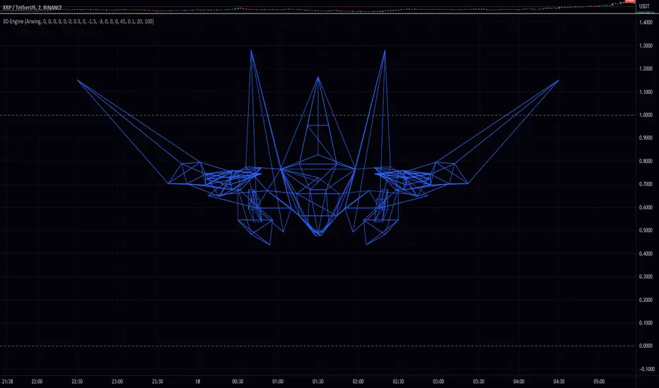
Trail3D is a first class streaming primitive built for visualizing two correlated time series as a 3D ribbon evolving through time. You give it a rolling buffer capacity and push (u, v) samples bar by bar; the primitive maintains the buffer, builds the ribbon geometry, and renders it inside a normalized bounding cube so the path always fits cleanly in view regardless of the underlying data range.
Under the hood, Trail3D is a coordinated bundle of polylines: one for the main ribbon, two for optional shadow projections onto the back wall and floor, and one for the wireframe cage. All four are depth sorted and occlusion clipped against the rest of the scene, and the primitive auto normalizes incoming samples against the rolling window's min/max so streaming data always fills the cube without manual scaling.
This enables a class of visualizations that would otherwise require dozens of polylines and manual buffer management: phase space portraits, Lissajous figures, oscillator pair correlations, attractor trajectories, and any "two indicators evolving together over time" study. The demo above shows a sine and cosine pair pushing samples each bar to trace a clean spiral inside the cage, the same pattern you would use to plot RSI vs MFI, momentum vs volatility, or any custom (u, v) signal pair.
A full streamed scene is a handful of lines:
//@version=6
indicator("Pine3D - Trail3D", overlay = false, max_polylines_count = 100, max_lines_count = 500, max_labels_count = 500)
import Alien_Algorithms/Pine3D/1 as p3d
var p3d.Scene scene = p3d.newScene()
var p3d.Trail3D trail = na
if barstate.isfirst
trail := p3d.trail3D(220.0, 200, color.yellow)
.cage(true)
.axisLabels("sin", "cos", color.white)
trail._uProj.col := #00ffff69
trail._vProj.col := #ff00ff71
scene.add(trail)
scene.camera.orbit(215.0, 20.0, 360.0)
float phase = bar_index * 0.15
float sinX = math.sin(phase) * 100.0
float cosY = math.cos(phase) * 100.0
if barstate.isconfirmed
trail.pushSample(sinX, cosY)
p3d.render(scene)
🔷 BARS3D: CATEGORICAL 3D BAR CHARTS
bars3D() turns any series of values into a fully lit, depth sorted 3D bar chart in a single call. Each bar is height mapped to its value, color graded between a low and high color, and packed into one combined mesh with per bar depth grouping so individual bars sort correctly even inside the merged geometry. The companion updateBars() mutator refreshes heights, colors, and labels in place every bar without rebuilding geometry, making it suitable for live rankings, rolling windows, and animated comparisons.
The chainable barLabels(catNames, valNames) helper attaches category labels at the base of each bar and value labels at the top, both depth sorted with the rest of the scene. Category labels are set once at build time, while value labels can be passed to updateBars(values, valLabels = ...) each frame to reflect live data. Combined with wireGrid() for the floor and a contour surface() in the background, bars3D() becomes the centerpiece of dashboards comparing assets, sectors, timeframes, or any categorical metric.
Negative values are handled automatically: bars below zero extrude downward from the base plane with reversed face winding, so signed series like PnL, delta, or momentum histograms render correctly without any extra setup.
A complete labeled bar chart is just a few lines:
//@version=6
indicator("Pine3D - Bars3D", overlay = false, max_polylines_count = 100, max_lines_count = 500, max_labels_count = 500)
import Alien_Algorithms/Pine3D/1 as p3d
var p3d.Scene scene = p3d.newScene()
var p3d.Mesh bars = na
array values = array.from(volume - volume , volume - volume , volume - volume , volume - volume , volume - volume , volume - volume )
array names = array.from("ΔV0", "ΔV-1", "ΔV-2", "ΔV-3", "ΔV-4", "ΔV-5")
if barstate.isfirst
bars := p3d.bars3D(values, 30.0, 30.0, 10.0, color.blue, color.red, 200.0)
.barLabels(names)
scene.add(bars)
p3d.wireGrid(scene, 300.0, 300.0, 6, 6, color.new(color.gray, 80))
scene.camera.orbit(215.0, 25.0, 360.0)
if barstate.islast
bars.updateBars(values)
p3d.render(scene, lighting = true)
Omitting valLabels in updateBars() tells the engine to auto format each numeric value via str.tostring() . Pass valLabels only when you need custom strings.
🔷 SCATTER CLOUDS: POINTS IN 3D SPACE
Pine3D treats scatter clouds as a first class use case without needing a dedicated scatter API. Because Label3D is the primitive and scene.add(array) is a single batch operation, you can scatter up to 500 points anywhere in 3D space, each with independent color, symbol, size, and tooltip , and have them depth sorted and occlusion clipped against the rest of the scene automatically.
Each point is a fully addressable Label3D with mutable fields. You can change position , textColor , bgColor , labelStyle (any label.style_* glyph including circles, squares, diamonds, triangles, crosses, arrows, flags), labelSize (any size.* preset), and text per point per bar. The renderer reads these mutations every frame, so animation is just direct field assignment.
This unlocks a wide class of visualizations: clustered data scatter, K means visualizations, particle systems, parametric surfaces sampled as point clouds, gradient colored attractors, multi class classification overlays, and structured curves like the demo above. The double helix demo plots two intertwined parametric strands as ~500 points with alternating colors and per point sizing, all inside the standard scene.add(array) pipeline.
The pattern is straightforward: build the array once in barstate.isfirst , add it to the scene, then mutate point fields per bar to animate.
//@version=6
indicator("Pine3D - Scatter Cloud", overlay = false, max_polylines_count = 100, max_lines_count = 500, max_labels_count = 500)
import Alien_Algorithms/Pine3D/1 as p3d
var p3d.Scene scene = p3d.newScene()
var array points = array.new()
if barstate.isfirst
for i = 0 to 499
p3d.Vec3 pos = p3d.vec3(0.0, 0.0, 0.0)
points.push(p3d.Label3D.new(position = pos, txt = "•"))
scene.add(points)
scene.camera.orbit(35.0, 20.0, 400.0)
if barstate.islast
for i = 0 to points.size() - 1
float t = i * 0.05 + bar_index * 0.01
p3d.Label3D pt = points.get(i)
pt.position := p3d.vec3(80.0 * math.cos(t), i * 0.4 - 100.0, 80.0 * math.sin(t))
pt.textColor := i % 2 == 0 ? color.aqua : color.fuchsia
p3d.render(scene)
----------------------------------------------------------------------------------------------------------------
🔷 TWO LAYER ARCHITECTURE
Pine3D ships as a clean, two layer library:
🔸 Layer 1 - DIY API. First principle building blocks ( Vec3 , Mesh , Camera , Light , Scene , plus world space overlay primitives) for total creative control. Author your own geometry, camera behavior, lighting setup, and scene graph from scratch.
🔸 Layer 2 - High Level Helpers. Production ready wrappers like surface() , bars3D() , trail3D() , updateBars() , updateSurface() , sphere() , torus() , cylinder() , and wireGrid() , plus chainable contour helpers gridBox() and gridLabels() that wrap the primitives into a few lines of code. Scatter clouds use the standard Label3D primitive directly.
The object model is chainable and scene oriented, so complex setups still read cleanly.
🔷 FEATURE LIST
Contour Surface Rendering - The most powerful 3D surface engine ever released for Pine Script. Render tens of thousands of polygon equivalent faces using a single polyline per contour band, delivering smooth, continuous terrain with natural ridges and valleys.
Adaptive Rail Sharing - Solid meshes drawn with the default linefill backend reuse one edge line between adjacent coplanar faces, averaging roughly 1.6 lines per face instead of the naive two, pushing practical mesh capacity up to ~360 faces depending on topology.
Interior Face Culling on Merge - mergeMeshes(meshes, removeInterior = true) detects coincident faces with opposing normals and strips them, so voxel style scenes (stacked cubes, block walls, lattice geometry) ship only their exterior shell and spend no budget on hidden interior faces.
True Perspective Camera System - Full 3D camera with position, target, fov, and orbit() controls. Supports cinematic camera movement, lookAt by mesh tag, and realistic depth.
Real Time Lighting and Shadows - Directional and point lights with configurable ambient, shadow strength, self shadowing, and a spatial grid acceleration structure for fast shadow queries.
High Performance Update System - updateSurface() and updateBars() let you animate massive datasets bar by bar without rebuilding geometry, keeping CPU usage minimal.
Rich Primitive Library - Cubes, cuboids, spheres, cylinders, tori, pyramids, planes, discs, circles, custom meshes, and the groundbreaking bars3D() with automatic labels.
Streamed Trail Primitive - trail3D() maintains a rolling buffer of (u, v) samples and renders them as a 3D ribbon inside a bounding cube, with optional projections onto the back wall and floor and a wireframe cage.
Depth Sorted Overlays - 3D labels, lines, polylines, wire grids, and trails, all correctly occluded and painter sorted against the rest of the scene.
Professional Contour Helpers - gridBox() and gridLabels() automatically add clean bounding boxes and axis titles, ticks, and series names that refresh on every updateSurface() call.
Tag Based Scene Graph - Every Mesh , Label3D , Line3D , and Polyline3D can carry a string tag. Scene exposes getMesh() , getLabel() , getLine() , getPolyline() , lookAt() , and remove() by tag, turning your scene into a lookup by name graph instead of an index juggling exercise.
Chainable, Intuitive API - Everything is designed for maximum readability and speed of development. Build complex scenes in just a few lines.
Production Ready Optimizations - World vertex caching, view projection caching, face preprocessing cache, shadow grid cache, and contour geometry cache, all managed automatically.
----------------------------------------------------------------------------------------------------------------
🔷 THE RENDERER
Every frame is produced by a single call to render(scene, ...) . The renderer runs the full pipeline: world transform, camera transform, back face culling, occlusion culling, depth sort, directional or point lighting with shadows, and perspective projection.
⚠ render() clears the entire chart drawing pool at the start of every call - every polyline , line , label , and linefill on the chart is deleted before Pine3D redraws, not just the ones it created. If you mix Pine3D with manual label.new() , line.new() , or similar calls, those drawings must be emitted after render() or they will be wiped every frame.
🔸 Setup Requirements. Pine3D consumes polylines, lines, and labels simultaneously, so your indicator() declaration must raise all three budgets, and the library must be imported under an alias:
indicator("My 3D Scene", overlay = false,
max_polylines_count = 100,
max_lines_count = 500,
max_labels_count = 500)
import Alien_Algorithms/Pine3D/1 as p3d
🔸 render() parameters.
maxFaces (int, default 100). Hard cap on solid faces drawn per frame. Contour bands, wireframe edges, labels, lines, and overlay polylines are not counted against this cap, and are bounded only by TradingView's global 100 polyline / 500 line / 500 label budgets.
culling (bool, default true). Enable back face culling.
lighting (bool, default false). Enable diffuse shading. Reads scene.light if set; otherwise falls back to the render() args.
lightDir (Vec3). Overrides scene.light.direction when provided. Points toward the light.
ambient (float, default 0.3). Minimum brightness for shadowed faces (0.0-1.0).
wireframe (bool, default false). Force outline only output for the entire scene.
occlusion (bool, default true). Sparse raster pass that drops hidden faces before drawing. Major perf win on dense scenes.
occlusionRaster (int, default 768). Raster resolution of the occlusion buffer. Lower = faster but coarser; higher = stricter hidden face rejection.
Explicit render() args always win over scene.light , which makes render() the right place for ad hoc, per frame lighting tweaks.
----------------------------------------------------------------------------------------------------------------
🔷 MESH DRAWING MODES
Two independent axes control how a mesh appears on the chart:
🔸 Style (via mesh.setStyle(...) ) - what gets drawn:
"solid" . Filled faces. Default.
"wireframe" . All edges, no fill. Shows interior geometry.
"wireframe_front" . Only front facing edges. Cleaner silhouette for convex meshes.
🔸 Draw Mode (via mesh.drawMode ) - which TradingView primitive carries the solid faces:
"linefill" (default). Uses the line and linefill budgets. An adaptive rail sharing optimization reuses one edge line between adjacent coplanar faces, pushing practical capacity up to ~360 faces per mesh depending on topology. Supports in place updates via updateSurface() and updateBars() . Rails are drawn transparent, so solid faces in this mode have no visible outline - use a wireframe style or "poly" drawMode if you need stroked edges. Recommended for all new code.
"poly" . Legacy polyline backend. Capacity ~100 faces, no in place updates, but renders the face outline using mesh.lineStyle and mesh.lineWidth . Use only when you need styled solid face outlines.
Wireframe styles always render with line primitives regardless of drawMode. Stroke width and style on edges (and on poly mode face outlines) come from mesh.lineWidth and mesh.lineStyle , which you mutate by direct field assignment.
----------------------------------------------------------------------------------------------------------------
🔷 QUICK START
The best practice lifecycle is simple:
Create one persistent Scene with newScene() .
Build meshes and helper overlays once in barstate.isfirst .
On later bars, mutate objects in place with transforms or helper mutators like updateBars() and updateSurface() .
Call render(scene, ...) once per frame. It automatically clears the previous chart drawings.
A complete, lit, animated 3D scene is still a handful of lines:
//@version=6
indicator("My First 3D Scene", overlay = false, max_polylines_count = 100, max_lines_count = 500, max_labels_count = 500)
import Alien_Algorithms/Pine3D/1 as p3d
var p3d.Scene scene = p3d.newScene()
var p3d.Mesh sun = na
if barstate.isfirst
scene.setLightDir(1.0, -1.0, 0.5).setAmbient(0.3)
sun := p3d.sphere(50.0, 16, 12, color.orange).setTag("sun")
scene.add(sun)
p3d.wireGrid(scene, 300.0, 300.0, 6, 6, color.new(color.gray, 80))
scene.camera.orbit(35.0, 25.0, 220.0)
if barstate.islast
sun.rotateBy(0.0, 1.5, 0.0)
p3d.render(scene, lighting = true)
----------------------------------------------------------------------------------------------------------------
🔷 RECOMMENDED USAGE PATTERN
Use your Scene and major meshes in var .
Build geometry once in barstate.isfirst .
Use updateSurface() and updateBars() on later bars instead of rebuilding meshes.
Use scene level helpers like wireGrid() when you want overlays added immediately.
Use trail3D() when you want a streamed oscillator style path with built in wall projections and cage geometry.
For scatter clouds, build an array once, hand it to scene.add(pts) , then mutate pt.position , pt.textColor , etc. each bar to animate.
Use mesh level gridBox() and gridLabels() (contour) and barLabels() (bars) to attach overlays to the mesh setup chain. They are drained into the scene by scene.add(mesh) .
🔷 CONSIDERATIONS
scene.clear() vs render(). scene.clear() removes objects from the scene graph (meshes, labels, lines, polylines). render() only clears the previous frame's TradingView drawings and redraws from the current scene graph. You almost never need scene.clear() in the build once and update pattern.
Global scope series for updateSurface() / updateBars(). If your data uses Pine's history operator ( ) or calls functions like ta.rsi() , ta.atr() , request.security() , those must be declared at global scope so Pine tracks their bar by bar history. Calling them inside barstate.islast produces inconsistent results or compiler errors.
gridLabels() tick values auto refresh. When you call updateSurface() , any tick value labels created by gridLabels() are automatically updated to reflect the new data range. Axis titles and positions stay constant. You don't need to rebuild them.
barLabels() value labels via updateBars(). Create category labels once with mesh.barLabels(catNames) at build time, then pass valLabels to updateBars() on each frame. Value labels are refreshed automatically. Don't call barLabels() again.
Lighting convenience methods are chainable. scene.setLightDir() , setLightPos() , setLightMode() , setAmbient() , setShadowStrength() , and showLightSource() all return Scene and can be chained: scene.setLightMode("point").setLightPos(0, 200, 150).setAmbient(0.25) .
Mesh transforms return Mesh. moveTo() , moveBy() , rotateTo() , rotateBy() , scaleTo() , scaleUniform() , setTag() , setStyle() , setColor() , show() , hide() all return Mesh for chaining: mesh.moveTo(0, -20, 0).rotateTo(0, 45, 0).setStyle("solid") .
Degrees vs radians. rotateTo() and rotateBy() on Mesh expect degrees. The low level Vec3.rotateX/Y/Z() methods expect radians.
scene.lookAt() is tag only. scene.lookAt(t) accepts a string tag and points the camera at that mesh. To aim the camera at an arbitrary Vec3 , call scene.camera.lookAt(vec) directly.
remove(tag) removes one object. The search order is meshes, then labels, then lines, then polylines, and the first hit wins. Avoid reusing tags across primitive types if you intend to delete by tag.
Shadow grid acceleration is directional light only. The spatial shadow grid is only built when lightMode == "directional" . Point lights fall back to a linear O(M) scan, so heavy shadow scenes are fastest in directional mode.
guiShift and yOffset. scene.guiShift and scene.yOffset position the 3D viewport on the chart without consuming historical bar slots. Increase guiShift to push the scene rightward into future bar space; adjust yOffset to slide it vertically in price units.
bar_time projection. All chart drawings are emitted with xloc.bar_time , so the scene can sit arbitrarily far left or right of bar_index without forcing Pine to extend its history buffer. This is what keeps the engine stable on long charts and future projected scenes.
barLabels() without values. When you call mesh.barLabels(catNames) and omit value labels, every later updateBars(values) auto formats the numeric values via str.tostring() . Pass valLabels only when you need custom strings.
Direct mesh.vertices mutation requires invalidateCache(). Transform mutators ( moveTo , rotateBy , scaleTo , etc.) invalidate the world vertex cache on their own. Only raw index writes like mesh.vertices.set(i, newVec) need a manual mesh.invalidateCache() call to force re-projection. Skipping it will make the renderer draw stale geometry.
Drawing budgets fail silently. If a scene emits more than 100 polylines, 500 lines, or 500 labels in a single frame, TradingView silently drops the overflow without raising a runtime error. Missing geometry almost always means a budget overrun - lower maxFaces , drop a contour level, or simplify overlay primitives to bring the frame back inside the caps.
render() deletes non Pine3D drawings too. Every render() call clears polyline.all , line.all , label.all , and linefill.all before redrawing. Any manual label.new() , line.new() , etc. issued before render() in the same frame will be wiped. Issue custom drawings after the render call if you need them to persist.
mergeMeshes() preserves depth grouping. When every source mesh passed into mergeMeshes() has the same vertex and face count (e.g. identical primitives in a voxel grid), the merged mesh auto derives depth group boundaries so the combined geometry still sorts correctly per original instance. Mixing primitives with different topologies disables the grouping.
CPU timeouts: knobs to turn. Pine Script enforces a per bar execution budget, and dense scenes can trip it before the drawing budget ever does. If a scene compiles but times out at runtime, reach for these levers in order: lower occlusionRaster (e.g. 768 -> 384) for the biggest single perf win, reduce maxFaces to cap the solid face pool, drop levels on contour surfaces, simplify sphere/torus segment counts, and gate heavy work behind barstate.islast so history bars only build geometry rather than render it.
----------------------------------------------------------------------------------------------------------------
🔷 MORE EXAMPLES
The following scenes were all built entirely in Pine Script™ v6 using Pine3D as the rendering layer. They exist to demonstrate that the library is a real engine capable of complex, production grade visualizations.
🔸 4D Hypercube (Tesseract). A rotating tesseract, projected from 4D to 3D to 2D in real time using a custom 4D rotation matrix layered on top of Pine3D's standard projection pipeline.
🔸 Solar System. Following the publication of my 3D Solar System back in 2024, which introduced new graphical rendering concepts into Pine Script, we have seen a wave of various interpretations of the underlying vector classes, ranging from tutorials to niche specific integrations using hardcoded math. It became clear that a unified architecture was needed, one that would lower the barrier to entry while simultaneously handling the optimization process, which is both complex and error prone to do manually.
That architecture is what Pine3D delivers. Below is a re-creation of the classic 3D Solar System rebuilt entirely on top of the library. It uses a fraction of the original code , renders roughly 5x faster , and adds real lighting cast directly from the Sun , all while consuming only a third of the available drawing budget thanks to the occlusion and culling mechanisms Pine3D handles out of the box.
----------------------------------------------------------------------------------------------------------------
🔷 API REFERENCE
🔸 Top Level Entry Points. newScene() creates a ready to use Scene with a default camera and light. render(scene, ...) draws the current frame and auto clears the previous frame's chart drawings; see the Renderer section above for the full parameter list. vec3(x, y, z) creates a Vec3. colorBrightness() is an exported color utility helper.
🔸 Mesh Factories.
Primitives - cube() , cuboid() , pyramid() , plane() , sphere() , cylinder() , torus() , grid() , disc() , circle() for ready made geometry.
customMesh(verts, faces) - Low level escape hatch for authoring your own topology.
mergeMeshes(meshes, tag, removeInterior) - Bakes transforms and combines many meshes into one. With removeInterior = true , coincident faces with opposing normals (e.g. shared walls between adjacent cubes in a grid) are culled so only the exterior shell survives, a major optimization for dense voxel style scenes.
surface(heights, size, lowCol, highCol, levels, axisX, axisZ) - Creates a contour surface mesh.
bars3D(values, barWidth, barDepth, spacing, lowCol, highCol, maxHeight) - Creates a combined 3D bar chart mesh; add labels with the chainable barLabels(names, values) method.
🔸 UDT Constructors. Overlay primitives and face descriptors are plain UDTs. Because these types have many fields, always instantiate them with named arguments rather than positional, e.g. Label3D.new(position = pos, txt = "•") :
Face - fields: vi (array of vertex indices into the parent mesh), col . Used when authoring customMesh() topology; every face must have at least 3 indices and should be planar.
Label3D - fields: position , txt , textColor , bgColor , labelStyle , labelSize , fontFamily , tooltip , visible , tag . Only position is required.
Line3D - fields: start , end , col , width , visible , tag , lineStyle .
Polyline3D - fields: points , col , fillColor , width , closed , visible , tag , lineStyle .
Vec3.new(x, y, z) or the vec3(x, y, z) shorthand.
🔸 Trail Primitive. trail3D(size, capacity, trailCol, minSamples) creates a streamed Trail3D primitive with a main trail, two projection polylines, and a cage polyline. capacity is internally clamped to 300 samples to keep the rolling buffer inside Pine's execution budget; passing a larger value silently resolves to 300. minSamples (default 60) is the sample count at which the cage reaches its full cube width: below that the cage stays cube shaped and samples stretch across it; above that the cage grows rightward at a fixed step until capacity is hit. scene.add(trail) registers the sub primitives into the scene. Trail3D methods: pushSample() , axisLabels() , cage() , moveTo() , show() , hide() .
🔸 Mesh Methods.
Transform - moveTo() , moveBy() , rotateTo() , rotateBy() , scaleTo() , scaleUniform() .
Appearance - setColor() , setFaceColor() , setStyle() , show() , hide() , setTag() .
Stroke styling (direct) - mesh.lineWidth := 3 and mesh.lineStyle := line.style_dashed control width and style of every visible mesh edge in wireframe modes and the outline of solid faces in drawMode = "poly" .
Shadow opt out (direct) - mesh.castShadow := false excludes the mesh from shadow casting while still receiving light. Useful for ghost overlays, debug geometry, or semi transparent meshes you do not want occluding the scene.
Lifecycle - clone() , faceCount() , invalidateCache() .
Data mutation - updateSurface() and updateBars() refresh persistent meshes in place. updateBars() refreshes any bar label positions automatically; pass catLabels / valLabels to also update the text.
Contour helpers - gridBox() and gridLabels() queue overlays on the mesh and hand them to the scene when you call scene.add(mesh) .
Bar helpers - barLabels() is chainable on a bars3D() mesh and queues its category and value labels for the next scene.add(mesh) .
Note: rotateTo() and rotateBy() expect degrees. The low level Vec3.rotateX/Y/Z() methods work in radians.
🔸 Scene Methods.
Lighting - setLightDir() , setLightPos() , setLightMode() , setAmbient() , setShadowStrength() , showLightSource() .
Scene graph - add(mesh) , add(label) , add(array) , add(line) , add(polyline) , add(trail) , remove(index) , remove(tag) , clear() .
Lookup and navigation - getMesh() , getLabel() , getLine() , getPolyline() , lookAt() , totalFaces() .
Cache control - invalidateLightCache() after mutating light direction or scene bounds externally; invalidateAllCaches() to also invalidate every mesh's world vertex cache (use after directly mutating mesh.vertices ).
Note: scene.clear() clears the scene graph itself. render() only clears the previous frame's TradingView drawings.
🔸 Camera Methods. setPosition(x, y, z) moves the camera. lookAt(x, y, z) / lookAt(vec3) points at a world space target. orbit(angleX, angleY, distance) does a spherical orbit around the current target. setFov(val) sets the perspective scale factor. Camera fields ( position , target , fov ) are also directly mutable via assignment when you need to tune them outside the provided setters, e.g. scene.camera.fov := 1200.0 .
🔸 Light Field Mutation. In addition to the scene level convenience setters, every field on scene.light is directly mutable for fine grained tuning: scene.light.selfShadow := true enables self shadowing, scene.light.shadowBias := 0.2 adjusts the shadow acne offset, scene.light.shadowStrength and scene.light.ambient are also exposed. Mutate them after newScene() or between frames; the renderer reads them every call.
🔸 Vec3 Methods. Core math: add() , sub() , scale() , negate() , dot() , cross() , length() , normalize() , distanceTo() , lerp() . Rotation and helpers: rotateX() , rotateY() , rotateZ() , copy() , toString() .
🔸 Overlay Primitive Methods.
Label3D - moveTo() , moveBy() , setText() , setTextColor() , setTooltip() , show() , hide() , setTag() .
Line3D - setStart() , setEnd() , setPoints() , setColor() , show() , hide() , setTag() .
Polyline3D - setColor() , show() , hide() , setTag() .
Every UDT field is mutable via direct assignment for properties without a chainable setter:
Label3D - bgColor , labelStyle (label.style_*), labelSize (size.*), fontFamily (font.family_*), visible .
Line3D - width , lineStyle (line.style_solid / _dashed / _dotted / _arrow_left / _arrow_right / _arrow_both), visible .
Polyline3D - width , lineStyle (line.style_solid / _dashed / _dotted only; arrow styles are not supported by TradingView's polyline primitive), fillColor , closed , visible .
Mutations are read per frame by the renderer, so they animate freely.
🔸 High Level Scene Helpers. wireGrid(scene, w, d, divX, divZ, col) adds a depth sorted ground grid. scene.add(array) adds a batch of labels in one call - the idiomatic way to push a scatter cloud into the scene.
🔸 Mesh Level Chainable Overlays. mesh.barLabels(names, values, ...) adds category and value labels on a bars3D() mesh. mesh.gridBox(col, divs) adds a wireframe bounding box cage on a surface() mesh. mesh.gridLabels(col, xName, yName, zName, ticks, fmt) adds axis titles and tick value labels on a surface() mesh; tick values auto refresh on updateSurface() . All three are queued on the mesh and drained into the scene by scene.add(mesh) .
----------------------------------------------------------------------------------------------------------------
This work is licensed under (CC BY-NC-SA 4.0) , meaning usage is free for non-commercial purposes given that Alien_Algorithms is credited in the description for the underlying software. For commercial use licensing, contact Alien_Algorithms
3d
Liquidity Surge Forecast with Markov Chains [TechnicalZen]Clear direction from Markov Chains confirmed projections.
Publishing this v3 with all the enhancements users desired and more. Thank you for your feedback.
What This Is
A 3D liquidity-and-momentum visualization that tells you where the market is heading right now, how long the current state is likely to hold, and when the next regime change is expected — all backed by a 2nd-order Markov chain that learns from your chart's own history.
Two independent systems — Money Flow (MFI-driven) and Price Current (Hull-VWMA or signed-ADX) — render as layered dotted carpets inside a bounded 3D box. When both systems agree on direction AND the Markov chain confirms, a whale surfaces — 🐳 bullish, 🐋 bearish. Chop gets a shark 🦈. Sideways drift gets a crab 🦀. And when the Markov chain predicts an imminent regime transition, a small hatchling whale appears before confluence forms.
The Current State row tells you, in one line, exactly what to expect next.
━━━━━━━━━━━━━━━━━━━━━━━━━━━━━━━━━━━
Built On
Money Flow Dynamics Forecaster 3D — the original 3D layered-terrain architecture, MFI/RSI momentum carpet, Hull-VWMA price current carpet, slope-extrapolated forecast, rider + whale system.
Same 3D engine. Same dual-system confluence as the foundation. Then: regime classification, Markov statistical learning, current-state intelligence, and a live win-rate scoreboard on top.
━━━━━━━━━━━━━━━━━━━━━━━━━━━━━━━━━━━
Clear Direction — At A Glance
Most indicators show you lines and ask you to interpret. This one tells you plainly, in a single dashboard row:
What regime you're in right now — 🐳 Bull, 🐋 Bear, 🦈 Chop-zone, or 🦀 Sideways
How long it's been held — in bars
Whether the regime is BALANCED or IMBALANCED — based on the Markov chain's next-bar probabilities
When the next regime change is expected — in bars, computed from the stay-probability
Which direction the market leans next — the highest-probability non-current state
Example readouts:
"Current State: 🐳 Bull held 5b · IMBALANCED — stay 68%, change expected in ~3b · next lean: 🦀 Sideways"
"Current State: 🦀 Sideways held 12b · BALANCED — change imminent · next lean: 🐳 Bull"
"Current State: 🐋 Bear held 2b · IMBALANCED — stay 82%, change expected in ~5b · next lean: 🦀 Sideways"
No interpretation required. You read the line, you know where you are, you know what to expect.
━━━━━━━━━━━━━━━━━━━━━━━━━━━━━━━━━━━
New Features — And Why Each Exists
1. Current State intelligence row
Why: Confluence indicators tell you WHEN a signal fires. They don't tell you "how solid is the current regime," "is a change coming," or "how long do I have before conditions flip." The Current State row answers all three in one glance.
The balanced / imbalanced distinction matters most:
BALANCED — the three next-bar probabilities are close to 1/3 each. No clear direction. A regime change is imminent (could go anywhere). Trade lighter, wait for resolution.
IMBALANCED — one direction dominates. Regime has a preferred path. The stay-probability tells you how long it's likely to persist; the next-lean tells you which direction it will tilt when it does flip.
The expected-bars-to-change is a geometric distribution mean: 1 / (1 − P(stay)). If a regime has 80% stay probability, it's expected to persist ~5 more bars. If 33%, it's expected to flip in ~1.5 bars.
2. 2nd-order Markov chain regime predictor
Why: the original whale logic was reactive — it fires after confluence forms. Markov is predictive — it learns your instrument's transition habits and uses them to gate and anticipate whale signals.
Pure statistics, no black box:
2nd-order — predicts the next regime from the pair of previous regimes, not just one. Captures patterns like "Chop → Sideways → 68% Bull next" that a 1st-order chain would miss.
Laplace smoothing (α=1) — every transition count gets a +1 pseudocount before normalization. Prevents "never observed → 0% forever" failure. Standard in real statistics.
Exponential recency decay — newer transitions count more than old ones (default 0.995/bar). Markets drift; stale history shouldn't dominate current prediction.
Duration conditioning — separate transition matrices for "current state held <5 bars" vs "held ≥5 bars." Regimes behave differently after they've been running. Real statistical sub-populations.
Confidence gating — if the current context has fewer than 10 observations, predictions are flagged low-n . No fabricated probabilities.
Maximum useful substance without gimmick. 3rd-order Markov would need thousands of regime transitions per cell to converge — doesn't happen on typical charts. 2nd-order is the ceiling before diminishing returns.
3. Dual-layer regime classification — Chop-zone 🦈 vs Sideways 🦀
Why: prior versions treated "not trending" as a single category. But there are two fundamentally different kinds of non-trending market:
🦈 Chop-zone — violent range-bound circling. Detected via classic Choppiness Index . Often precedes a sharp breakout.
🦀 Sideways — slow drift, flat angles across close/high/low at both short and long periods. Detected via angle consensus . Often indicates accumulation or distribution.
Showing them separately lets you read which kind of non-trending you're in. Different implications, different decisions.
4. Hatchling whales — pre-signal pre-whales
Why: the Markov chain lets us anticipate confluence before it forms. When the current state is Sideways AND Markov predicts Bull (or Bear) with confidence above the hatchling threshold, a small whale appears at the mid-forecast position — a heads-up that confluence is probabilistically coming.
Full whale (size.huge at forecast edge) = confluence is here now.
Hatchling whale (size.small at forecast mid) = confluence is probably coming soon.
Better entries on regime changes.
5. Markov-gated whale confirmation
Why: sometimes projected-confluence fires, but the instrument's historical pattern says "from this context, the opposite is more likely." That's exactly the setup a trader wants the indicator to filter out .
The gate is permissive — Markov blocks a whale only if it's confident AND its argmax points the opposite direction. Uncertainty or agreement = pass through. Reduces false confluence without over-filtering.
6. Regime-aware 4-column win-rate dashboard
Why: knowing how much time the instrument actually spends in each regime is as actionable as the signals themselves.
Four parallel columns:
🐳 Bull — confluence signals and win rate
🐋 Bear — same, opposite direction
🦈 Chop-zone — CI chop events and % of bars
🦀 Sideways — angle-sideways events and % of bars
If your instrument spends 80% of bars in Chop/Sideways, confluence will be rare — adjust timeframe or instrument. If Markov shows low-n on most bars, the matrix isn't populated yet — wait for more history before trusting predictions.
7. Session-aware for futures
Why: NQ, ES, CL and other overnight-session futures stamp their daily bar at session start , which is the previous calendar evening. Naive `dayofweek(time)` reads NQ's "Friday session" as Thursday. The indicator uses `time_close("D")` — the close of the daily bar, always on the trading date — so regime classification is correct for both cash equities (TSLA, SPY) and overnight futures (NQ, ES). Same indicator, any asset class.
8. Honest evaluation — next-signal MFE or directional close
Why: "close-at-N-bars" is dishonest. Price can move 2×ATR favorably then retrace — close-at-N logs that as a loss. MFE logs it as what it actually was.
Each signal is held pending until the next signal fires. It's a win if either:
The close at next-signal bar was directionally favorable vs entry, OR
The Maximum Favorable Excursion between the two signals reached the ATR-scaled threshold (default 0.5×ATR at entry bar)
Either qualifies. Transparent. Computed live. Disclaimer embedded in the dashboard footer.
━━━━━━━━━━━━━━━━━━━━━━━━━━━━━━━━━━━
How to Read the Dashboard
┌────────────────────────────────────────────────┐
│ Liquidity Surge + Markov · Win Rate │
├────────┬────────┬─────────────┬───────────────┤
│🐳 Bull │🐋 Bear │🦈 Chop-zone │🦀 Sideways │
│42 sigs │38 sigs │7 events │12 events │
│31 wins │24 wins │120 bars │45 bars │
│73.8% │63.2% │23% │8.6% │
├────────────────────────────────────────────────┤
│Markov Forecast Next: 🐳 52% · 🦀 31% · 🐋 17% │
├────────────────────────────────────────────────┤
│Current State: 🐳 Bull held 5b · IMBALANCED │
│ stay 68%, change expected in ~3b · next: 🦀 │
├────────────────────────────────────────────────┤
│⚠ Not financial advice · Learned on chart hist │
└────────────────────────────────────────────────┘
Reading order:
Column data — how Bull/Bear signals have performed, how much time is spent in each regime
Markov Forecast Next — next-bar regime probabilities (with sample-size confidence)
Current State — the single-line answer to "where am I and what's next"
Footer — disclaimer + config
━━━━━━━━━━━━━━━━━━━━━━━━━━━━━━━━━━━
How to Use
Load with defaults.
Wait for ~100-200 bars of history. The Markov matrix needs observations to learn.
Read Current State first. It tells you what to expect.
If BALANCED → expect a regime change, trade light.
If IMBALANCED + change in ~N bars → plan around that window.
Watch for 🐳 / 🐋 full whales at the forecast edge — confluence + Markov confirmed.
Watch for small hatchling whales at forecast mid-point — Markov's early prediction of confluence coming.
Respect 🦈 (chop-zone) and 🦀 (sideways). Don't fight the regime.
Tune Hatchling Threshold and Win Threshold (×ATR) to your instrument and style.
━━━━━━━━━━━━━━━━━━━━━━━━━━━━━━━━━━━
Best Paired With Smart Candle Structures
This indicator answers whether and when to trust the flow. Smart Candle Structures answers where to act. Together: right place, right moment, measurable conviction, regime-aware.
━━━━━━━━━━━━━━━━━━━━━━━━━━━━━━━━━━━
Key Settings
Time Span — past bars rendered + forecast horizon (default 15)
Momentum Source — MFI (default) or RSI
Oscillator Type — Hull-VWMA (default) or signed-ADX
Slope Lookback — bars for slope that fires whales (default 4)
Evaluation Window — bars after a signal to measure MFE (default 5)
Win Threshold (× ATR) — minimum favorable excursion as a multiple of ATR (default 0.5)
Gate Whale by Choppiness — master toggle for 🦈 / 🦀 filter
CI Length / CI Threshold — classic Choppiness Index tuning
Angle Short / Long Period — angle-based sideways lookbacks
Angle Trend / Sideways Threshold — angle degrees defining trending vs sideways
Use Markov Predictor — master toggle for the 2nd-order chain
Count Decay per Bar — recency weighting for Markov counts (default 0.995)
Hatchling Threshold — minimum Markov probability to fire pre-whale (default 55%)
Dashboard Text Size — Tiny / Small / Normal / Large / Huge
Camera — yaw / pitch / scales for the 3D view
━━━━━━━━━━━━━━━━━━━━━━━━━━━━━━━━━━━
Disclaimer
This is a visualization and analytical tool, not financial advice or a signal service. The Markov chain is trained on your chart's history — it describes what has happened on this instrument at this timeframe, not what will happen. Regime transition probabilities are learned estimates; past frequencies do not guarantee future outcomes. Markets are reflexive and can transition in ways the chain has never observed. Hatchlings, whales, sharks and crabs are visualizations of mathematical predictions — they do not constitute buy or sell recommendations. Trade with your own risk management. Every trade can lose.
The indicator echoes this disclaimer in its dashboard footer so you see it every time you read the chart. It's always there because it's always true.
━━━━━━━━━━━━━━━━━━━━━━━━━━━━━━━━━━━
Clear direction from learned regimes.
— TechnicalZen
Pine Script® indicator
Liquidity Surge Forecast with Win Rate [TechnicalZen]Publishing this v2 with Proven performance dashboard for scalpers.
What This Is
A 3D liquidity-and-momentum visualization with a built-in, MFE-verified win-rate dashboard.
Two independent systems — Money Flow (MFI-driven) and Price Current (Hull-VWMA or signed-ADX) — render as layered terrains inside a bounded 3D box. When both systems agree on direction, a whale surfaces: 🐳 bullish, 🐋 bearish. Every whale is tracked. Every outcome is scored. The dashboard prints the running win rate on your chart, on your instrument, on your timeframe. Live.
━━━━━━━━━━━━━━━━━━━━━━━━━━━━━━━━━━━
Built On Money Flow Dynamics Forecaster 3D
This is the next iteration. Same solid confluence-detection engine, rebuilt rendering, and a performance dashboard on top for visual proof of how the system is doing.
Improvements over v1:
Win-rate dashboard with ATR-scaled MFE — every 🐳 / 🐋 signal is now tracked and scored. Each signal resolves when the next one fires, judged by directional close or MFE ≥ 0.5 × ATR. No more hand-waving about "does this actually work."
Seamless carpet terrain — layered strips share color between fill and outline. No visible seams; the terrain reads as one continuous surface.
Dotted wave contours — each HMA layer traces as a dotted line along its depth, like isobars on a topographic map. Wave shape is visible at a glance.
Depth fog gradient — far Z layers tint toward atmospheric navy-violet. Real 3D depth perception without extra wireframe.
Dotted wireframe, emphasized horizon — box edges and grids are dotted (quieter), while the Y=0 tide line is kept solid and bold as the one structural anchor that should stand out.
Unified ADX-mode terrain — ADX mode now renders a proper 12-layer terrain (v1 fell back to a single-ribbon). Both oscillator modes share identical visual grammar.
Cleaner defaults — Yaw −20°, Pitch 15°, axis markers off, back-wall grid off, mesh columns removed. Less visual noise out of the box.
Bug fixes — ring-buffer wrap when Slope Lookback > Time Span ; ADX-mode second-signal for the emoji confluence check; dead inputs cleaned up.
If you're coming from v1, interpretation is identical — same riders, same whales, same color semantics. The new dashboard simply gives you a way to measure how often confluence actually pays off.
━━━━━━━━━━━━━━━━━━━━━━━━━━━━━━━━━━━
The Win-Rate Dashboard — Proof, Not Claims
Most indicators claim a success rate. This one measures it.
Every 🐳 / 🐋 signal is recorded at its first bar of entry and held pending — until the next signal fires. At that moment the indicator judges the previous signal by two criteria :
Directional close — did price close favorable at the next signal's bar? (bull: close > entry. bear: close < entry.)
MFE ≥ ATR threshold — did the favorable excursion between the two signals reach 0.5 × ATR (at the entry bar)? ATR multiplier is tunable.
Either criterion qualifies as a win. Direction alone is a win. MFE alone is a win. No fixed evaluation window — signals are judged against reality when the regime actually changes.
The threshold is volatility-relative : quiet instruments need small moves, volatile ones need larger moves. Always calibrated to the instrument, never arbitrary.
The dashboard shows:
Total bull and bear signals fired (resolved ones only — the most recent signal is pending until the next)
How many won
Rolling win rate, traffic-lit — green ≥ 60%, yellow 40–60%, red < 40%
Your ATR multiplier, printed right on the table
Why next-signal evaluation? Because fixed bar counts are arbitrary. A regime lasts as long as it lasts. When the next whale flips, the previous whale's journey is over — and that's the fair moment to judge it. Entry quality and regime persistence are both captured naturally.
The result: you don't trust marketing, you trust your own data . Every number is computed from your chart, right now, with your settings. Change the ATR multiplier, change the timeframe — the dashboard updates. This is how an indicator should prove itself.
━━━━━━━━━━━━━━━━━━━━━━━━━━━━━━━━━━━
The Signal
Confluence requires agreement between two fundamentally different witnesses:
Money Flow — volume-weighted momentum (MFI). 20 Hull-smoothed layers (HMA 3 → HMA 60). Detects accumulation or distribution before price has to move.
Price Current — volume-weighted directional pressure (Hull-VWMA 2-bar slope, or signed-ADX HMAs). 12 layers. Detects committed displacement of price.
Money Flow leads. Price Current confirms. When both middle-layer slopes point the same way, a whale fires. That is the signal worth trading — not a crossover, not a threshold break, but two independent systems aligning.
━━━━━━━━━━━━━━━━━━━━━━━━━━━━━━━━━━━
What You See
Layered dotted waves — each HMA smoothing horizon, stitched into a 3D carpet. Depth fog tints far layers into atmospheric haze for real 3D perception.
Forecast terrain — each layer slope-extrapolated with exponential decay into the future half of the box.
🏄♂ Surfer — rides the Money Flow leading edge (the impulse).
⛵ Sailboat — rides the Price Current leading edge (the trend).
🐳 / 🐋 Whale — surfaces at the forecast edge when both slopes agree. Confluence confirmed.
Dashboard — running win rate, always visible.
━━━━━━━━━━━━━━━━━━━━━━━━━━━━━━━━━━━
How to Use
Load with defaults. Switch chart to Volume Candles.
Check the dashboard — what is your current win rate on this instrument / timeframe?
Tune Win Threshold (× ATR) to match how strict you want the measurement to be — 0.3×ATR = loose, 0.5×ATR = balanced (default), 1.0×ATR = strict.
Watch for 🐳 or 🐋. They are rare by design.
On a whale, align with the direction. On no whale, stand aside. Let the dashboard keep scoring.
━━━━━━━━━━━━━━━━━━━━━━━━━━━━━━━━━━━
Best Paired With Smart Candle Structures
This indicator tells you whether and when to trust the flow. Smart Candle Structures tells you where to act — order blocks, fair-value gaps, liquidity sweeps, BOS / CHoCH zones.
Together: the right place, at the right moment, with a measurable win rate behind it.
━━━━━━━━━━━━━━━━━━━━━━━━━━━━━━━━━━━
Key Settings
Time Span — past bars rendered and forecast horizon (default 15)
Momentum Source — MFI (default) or RSI
Oscillator Type — Hull-VWMA (default) or signed-ADX
Slope Lookback — bars used to compute the slope that fires whales (default 4)
ATR Length — lookback for volatility scaling the win threshold (default 14)
Win Threshold (× ATR) — minimum favorable excursion between signals, as a multiple of ATR at the entry bar (default 0.5 × ATR)
Depth Fog Strength — atmospheric depth gradient on far layers (default 0.55)
━━━━━━━━━━━━━━━━━━━━━━━━━━━━━━━━━━━
Disclaimer
This is a visualization and analytical tool, not financial advice or a signal service. The dashboard measures what has happened on your chart; it does not predict what will. Markets are reflexive. Past performance does not guarantee future results. Trade with your own risk management. Every trade can lose.
━━━━━━━━━━━━━━━━━━━━━━━━━━━━━━━━━━━
Confluence you can measure.
— TechnicalZen
Pine Script® indicator
Temporal Volume Profile 3D [LuxAlgo]The Temporal Volume Profile 3D indicator is a spatial visualization tool that transforms historical volume data into a three-dimensional landscape, adding a time-depth dimension to traditional volume analysis.
By projecting volume across price (X), time (Y), and magnitude (Z), it allows traders to observe the evolution and migration of liquidity over time rather than viewing it as a static, aggregate value.
🔶 USAGE
The primary advantage of this script is its ability to reveal the "lifecycle" of volume nodes. While a standard Volume Profile (VP) squashes all historical data into a single 2D histogram, this tool slices the lookback period into distinct segments, creating a "terrain" where the most recent volume is in the foreground and older volume resides in the background.
🔹 Identifying Volume Migration
By observing the peaks of the volume mountains, you can see if the Point of Control (POC) is migrating. A POC shifting from the background (older) to the foreground (newer) indicates a trending consensus of fair value, whereas a consistent peak across all time slices suggests a long-term, stable support or resistance zone.
🔹 Price Proximity & Liquidity Interaction
The indicator includes a real-time price tracker that moves across the 3D terrain. If the current price enters a significant historical volume mountain, the tracker triggers a "Peak Warning," signaling that the price is entering a high-liquidity zone likely to cause consolidation or reversal.
🔹 The Paths of Least Resistance
Valleys in the 3D landscape represent Low Volume Nodes (LVNs). When price moves into a valley that has remained empty across multiple time slices, it indicates a lack of historical interest at those levels, often resulting in fast, "slippery" price action through those zones.
🔶 DETAILS
Standard Volume Profiles lose the "when" of volume accumulation. For example, a 2D profile might show a large volume peak at $100, but it cannot tell you if that volume was traded 200 bars ago or 5 bars ago. The Temporal Volume Profile 3D solves this by using a Painter's Algorithm to render slices of volume data along a depth axis.
🔹 3D Engine & Projection
The script uses a custom trigonometric projection engine allowing users to adjust the Yaw (rotation) and Pitch (tilt) of the landscape. This allows for a bird's-eye view to see the "map" of volume or a side-profile view to emphasize the height of the volume peaks.
🔹 POC Ridge Line
This feature connects the highest volume node of every time slice. This creates a continuous path through the mountains, providing a visual history of how the most significant price levels have changed over the selected lookback period.
🔶 SETTINGS
🔹 Volume Profile & Matrix
Lookback Bars: The total historical window used for the calculation.
Price Bins (Width): Determines the horizontal resolution (X-axis). Higher values provide more detailed price levels.
Time Slices (Depth): Determines how many segments the volume is divided into (Y-axis).
Terrain Smoothing: Blends adjacent volume nodes to create a more organic, mountain-like appearance.
🔹 Camera Projection
Yaw/Pitch: Controls the angle of the 3D projection.
Scale X/Y/Z: Adjusts the width, depth, and height of the volume mountains.
Offset X/Y: Moves the 3D object on the chart to prevent it from overlapping with current candles.
🔹 Style & Colors
Show Ridge Lines: Toggles the colored outlines for each time slice.
Mountain Fills: Enables the use of the background color to occlude lines, creating a solid 3D effect.
Show POC Ridge Line: Toggles the yellow line tracking the peak volume through time.
Peak Proximity Warning: Toggles the color change on the price tracker when entering high-volume zones.
Pine Script® indicator
Money Flow Dynamics Forecaster 3D [TechnicalZen]The art of swimming with the whales 🐳
What is this?
MFDF 3D provides a topological three-dimensional mapping of current market drivers and potential future trajectories.
is a visual analysis indicator that compresses several ideas into one spatial model: recent history, layer depth, directional amplitude, and short-term forward continuation.
Visually a three-dimensional momentum ocean where two independent systems — Money Flow (MFI-driven) and Price Current (Hull-VWMA-driven) — are rendered as layered terrains inside a bounded 3D box. Past history forms a waved carpet; the future is slope-extrapolated with exponential decay. When both systems agree, whales appear — 🐳 when the tide is rising, 🐋 when it's falling.
━━━━━━━━━━━━━━━━━━━━━━━━━━━━━━━━━━━
The Metaphor — Swimming With the Whales
Markets do not move on their own. They move because whales move them — large institutional players whose positions are too big to enter or exit in a single candle. A pension fund building a position, a market maker hedging a block, a macro desk rotating out of a sector — none of them can step in without leaving ripples.
When whales move, they leave two distinct footprints in the tape:
Money Flow — volume concentrated at favorable prices. You don't see it as a price change at first; you see it as buying pressure accumulating . MFI, weighted by volume, detects this before it becomes price.
Price Current — the volume-weighted tide. Once enough pressure accumulates, price itself has to drift in the direction the whale is pushing. Hull-VWMA slope tracks this.
Retail traders typically see only the second footprint — price moving. By then the whale is already positioned. Money Flow shows you the first footprint before price has to respond, which is why MFI leads VWMA in this indicator.
The goal is not to catch the whale — you can't. The goal is to see the ripples early enough to swim with the tide instead of against it. That's what "swimming with the whales" means: recognizing the institutional current and aligning with it, instead of fading it and getting dragged under.
━━━━━━━━━━━━━━━━━━━━━━━━━━━━━━━━━━━
The Fluid Dynamics
Every oscillator you've used is a single line. MFI is one line. RSI is one line. MACD is two lines and a histogram. They're flat because they pick one smoothing length and commit to it. You see where momentum is; you don't see its shape .
This indicator draws a family of 20 Hull-smoothed Money Flow variants simultaneously , each using a different HMA length (3, 4, 5, 6, 8, 10, 12, 14, 17, 20, 23, 26, 30, 34, 38, 42, 46, 50, 55, 60). Short HMAs foam at the surface, reacting instantly. Long HMAs move like glaciers. Stitched together across time and depth, they form a genuine fluid — ripples, waves, surges, cascades, turning-tides — not a line, a current.
The Hull-VWMA carpet is the same idea on a second dimension: 12 depth layers, each the 2-bar percentage slope of a Hull-smoothed Volume-Weighted Moving Average. This is your price current : where the volume-weighted tide is moving, independent of momentum.
Two independent Wireframes. Shared 3D box. When they agree, the whale arrives.
━━━━━━━━━━━━━━━━━━━━━━━━━━━━━━━━━━━
The 3D Box
Axes:
X — time (past bars left of center, forecast right)
Y — amplitude, signed ±100 (positive = bullish, negative = bearish)
Z — depth layer (each HMA length sits at a different depth)
Reference planes:
The translucent Y=0 plane is momentum neutrality — where MFI = 50, VWMA slope = 0. Wireframes rise above it when bullish, sink below when bearish.
The X=0 plane marks the current candle. Everything to the left is memory; everything to the right is forecast.
Nine labeled points (A–I) on the Y=0 plane let you orient instantly.
Riders:
🏄♂ — rides the leading edge of the Money Flow terrain (HMA 20 middle layer)
⛵ — rides the Price Current leading edge (Hull-VWMA slope in Hull-VWMA mode, signed-ADX HMA in ADX mode)
🐳 — breaches at the forecast end when both slopes are bullish
🐋 — dives at the forecast end when both slopes are bearish
━━━━━━━━━━━━━━━━━━━━━━━━━━━━━━━━━━━
Color Aesthetics
The color choices are not random — they carry semantic weight.
Money Flow terrain uses traffic-light logic:
Yellow at neutral (v ≈ 0)
Yellow → Green as bullish momentum grows
Yellow → Red as bearish momentum grows
Solid green above +50, solid red below −50
Hull-VWMA carpet uses a water palette:
Light blue at neutrality — still water
Light blue → Cyan as money flows in
Light blue → Maroon as money flows out
Transparency encodes magnitude: weak signals fade to nearly invisible, strong signals saturate. You read intensity at a glance, without staring at a number.
━━━━━━━━━━━━━━━━━━━━━━━━━━━━━━━━━━━
The Forecast
Past Wireframes tell you where you've been. The right half of the box projects where you're heading .
Each of the 20 + 12 = 32 HMA layers gets slope-extrapolated into the future:
future = current + slope · t · decay^t
slope is computed from the last N bars (default 4)
decay (default 0.92) is the honesty multiplier — the further out you go, the less confident the projection, so the slope contribution fades
All forecast values clamp to ±100 so they never escape the box
Rendered as translucent ghost terrain in the forecast half, colored with the same palette as the past but softer. You see the shape of projected momentum , not a point estimate.
When both the Money Flow middle-layer slope AND the Hull-VWMA middle-layer slope agree on direction, a whale surfaces at the forecast's far edge. This is confluence — two independent systems pointing the same way. That's the signal worth swimming toward.
━━━━━━━━━━━━━━━━━━━━━━━━━━━━━━━━━━━
The Two Riders — Surfer vs Sailboat
The two emojis on the present-boundary are not decoration. They represent two fundamentally different kinds of signal — and understanding the difference is the whole game.
🏄♂ The Surfer — rides the Money Flow terrain. Surfers feel the impulse : every short wave, every gust of buying or selling pressure, every sudden shift in volume-weighted momentum. Surfers are fast, reactive, sensitive. What the surfer tells you: "the wind just picked up" — or "it just died." This is the quick, leading signal.
⛵ The Sailboat — rides the Price Current carpet. Sailboats don't react to gusts; they set their course by the trend — the steady directional pressure of the volume-weighted tide pushing the boat one way or the other. Slow, deliberate, confirmed. What the sailboat tells you: "the current is actually carrying us this way now." This is the confirming, lagging signal.
These are two different kinds of information, not two views of the same thing:
The surfer sees the impulse before it matures into committed direction.
The sailboat confirms that the impulse has turned into real directional displacement.
When both agree — surfer AND sailboat pointing the same way — momentum builds faster than either signal could account for alone. That agreement is the proof that big money isn't just testing the waters; they're actually moving them. That's when a whale surfaces.
Surfer alone = wind, no commitment yet. An impulse without confirmation — interesting but unconfirmed.
Sailboat alone = drift, no fresh push. A trend without new pressure — may be tired.
Surfer + Sailboat = whale. Both fresh impulse and committed direction. Institutional participation confirmed.
━━━━━━━━━━━━━━━━━━━━━━━━━━━━━━━━━━━
Reading the Whales — What They Mean For Decisions
A whale is not a liquidity-grab signal. It is a confluence signal: both independent systems have agreed on direction at the same time.
🐳 — Money Flow and Price Current are both rising. Buyers are accumulating AND getting filled at progressively higher prices. This is sustained pressure, not a stop-hunt or a single-bar spike.
🐋 — Both falling together. Selling pressure AND price giving ground in lockstep.
No whale — the two systems disagree, or both are flat. Low-conviction zone.
Decision framework
🐳 → align long, don't fade. This is a conviction trade, not a reversal bet. Big money is actually pushing the tape, so size up with the tide instead of against it.
🐋 → exit longs or consider shorting. Don't buy the dip blindly — the volume-weighted price is confirming the sellers, not fighting them.
No whale → stand aside, or scale out of existing positions. Wait for confluence before committing fresh risk.
The mental model: "is big money actually moving the tape right now, or just shuffling?" Whale = pushing. No whale = shuffling.
━━━━━━━━━━━━━━━━━━━━━━━━━━━━━━━━━━━
Helpful Tip — Money Flow Leads Price Current
How to Use It in Practice
The best way to use the indicator is to read it in layers. It is not a one-glance yes or no system. Its advantage comes from helping the user see whether a move has internal support, whether the structure is broadening or thinning, and whether the present slope still has credible continuation.
• Start with orientation: Keep the default camera first. Learn where the zero plane is, where present time sits, and how positive and negative terrain occupies the box.
• Read the momentum terrain first: Look for height, curvature, and continuity across layers. A broad aligned rise or fall is stronger than a single sharp spike on only the fast layers.
• Check the oscillator carpet next: In Hull-VWMA mode, ask whether price-current slope supports momentum. In ADX mode, ask whether directional trend strength is building under the move.
• Inspect the forecast half: Use the ghosted forward half as a continuation sketch, not as a promise. Flattening structure, decaying height, or diverging layers often matter more than the exact projected endpoint.
• Use the whale as confirmation, not as the whole trade: The whale is most useful when it appears after the terrain has already become coherent, not when the picture is still fragmented and noisy.
Practical setup profiles
Fast tape
Suggested mode: MFI + Hull-VWMA
What to emphasize: Steeper terrain changes and quicker second-signal response.
Reading style: Use for intraday pulse and immediate continuation checks.
Cleaner swing structure
Suggested mode: RSI + Hull-VWMA
What to emphasize: Broader curvature and less volume sensitivity.
Reading style: Use when the user wants smoother rhythm and cleaner layer alignment.
Trend-strength confirmation
Suggested mode: MFI or RSI + ADX
What to emphasize: Whether directional pressure is actually strengthening underneath the move.
Reading style: Use when momentum looks attractive but may be structurally weak.
In practice, the Money Flow terrain (yellow/green/red) turns before the Hull-VWMA carpet (cyan/blue/maroon) . Volume-driven accumulation and distribution show up in MFI first — price only has to move afterwards to reflect what already happened underneath.
What to watch for:
Momentum terrain flipping color while the carpet is still flat → early warning . A whale sighting may be forming but is not yet confirmed.
Carpet starting to tilt the same way → confirmation building . Slopes are aligning.
🐳 / 🐋 appears at the forecast edge → confluence . Both systems point the same way. Act.
Read the terrain first. Wait for the carpet to catch up. Act on the whale.
━━━━━━━━━━━━━━━━━━━━━━━━━━━━━━━━━━━
Why This Is Different
Traditional oscillators answer: "what is momentum doing right now?"
This indicator answers:
What is money flow doing across every smoothing horizon at once? — the 20-layer Wireframe shows the full shape of momentum, not a single slice
What is the volume-weighted price doing independently? — the Hull-VWMA carpet is a second, independent witness
What do they predict together? — slope-extrapolated forecasts fill the future half; confluence emojis mark conviction
How strong is the signal? — opacity, saturation, and emoji presence are all quantitative encodings
No threshold to wait for. No line to cross. The ocean tells you where you are — and the whales tell you where it's heading.
━━━━━━━━━━━━━━━━━━━━━━━━━━━━━━━━━━━
Best Used With Volume-Weighted Candles
Switch your TradingView chart's bar type (top-left dropdown) to Volume Candles .
Here's why this matters: the Hull-VWMA layer is already volume-weighted mathematically. When the chart's candles are ALSO volume-weighted, every visible pixel speaks the same language — price, indicator terrain, and forecast are all reading the same volume-filtered reality.
Thin-volume wicks and gap-outs stop polluting the chart, so they stop polluting the forecast
🐳 / 🐋 confluence signals calibrate more cleanly because both the price action and the indicator see the same "what the volume actually cared about"
On plain OHLC candles the indicator still works — but low-liquidity price spikes can disagree with the terrain. On VWC they move in lockstep.
If you want one setup to remember: Volume Candles + this indicator + default settings . Swim with the whales.
━━━━━━━━━━━━━━━━━━━━━━━━━━━━━━━━━━━
Best Paired With Smart Candle Structures
This indicator answers one question: "Is big money flowing, and in which direction?" It does not answer: "At what price level should I enter, exit, or place my stop?"
For that you need structural context — the levels where the market has historically reacted. Smart Candle Structures (order blocks, fair value gaps, liquidity pools, break-of-structure / change-of-character zones) maps exactly those levels.
The two tools are complementary, not redundant:
Smart Candle Structures gives you WHERE — the structural level worth reacting at.
MFD Forecaster gives you WHETHER AND WHEN — is the flow actually supporting a reaction here, and is it committed enough to act on?
The ideal workflow:
Smart Candle Structures highlights a level worth watching (an unfilled order block, a liquidity sweep, a CHoCH break).
Price arrives at that level. You don't act yet.
Watch this indicator: is the surfer turning? Is the sailboat joining? Is a whale forming in the forecast half?
Structure + confluence = your trigger. Structure without confluence = low-conviction trap. Confluence without structure = direction without location.
Pair them and you have both legs of the trade: the right place, at the right moment, with conviction .
━━━━━━━━━━━━━━━━━━━━━━━━━━━━━━━━━━━
TradingView Chart Stretch — Feature, Not Bug
Pine drawings live in chart coordinates (bar_index × price), so they stretch with your chart. Most indicator authors fight this. We lean into it.
Horizontal zoom → bar spacing changes → the 3D box widens or tightens organically. Zoom in tight to inspect individual layer positions; zoom out to see broad wave cycles.
Pane height changes → vertical proportions adjust. Invisible ±50 anchor plots lock the Y range so the box never jumps when values move.
Emojis scale with the pane — surfers and whales always read clearly at any zoom.
The indicator breathes with your viewport . That's what a real 3D visualization should do in a chart environment. It's responsive by design, not despite itself.
━━━━━━━━━━━━━━━━━━━━━━━━━━━━━━━━━━━
Settings Overview
Core
Time Span — past bars rendered (default 15). Also the forecast horizon.
Momentum Source — MFI (volume-weighted, default) or RSI (pure price)
Momentum Length — 14 default
Rib Amplification — stretches the ribs vertically to fill the box
Oscillator (Hull-VWMA)
VWMA Length — default 30
HMA Length — default 20
Hull-VWMA Scale — amplifies the slope into ±100
Bull/Bear/Neutral Tint colors
Camera
Yaw — horizontal rotation (−180 to +180)
Pitch — vertical tilt (default 5° = eye-level)
Scale X / Y / Z — box proportions
Forecast
Slope Lookback — bars used to compute current slope (default 4)
Decay per Bar — how slope contribution fades into the future (default 0.92)
Display
Box Wireframe, Y=0 plane, Axis markers, Mesh wireframe, Grids (all togglable)
Show Emoji Markers — master toggle for all four emojis
Quick-Start Tips
Load with defaults.
Switch chart bar type to Volume Candles.
Watch for 🐳 and 🐋 — they're rare, by design. They mean confluence.
Read the color gradient — yellow is neutral, bright green / cyan is strong bull, red / maroon is strong bear.
Try yaw presets: 0 = front view, 45 = corner, 90 = side, 180 = back.
Lower time spans (10–15) for intraday, higher (25–40) for daily and weekly.
Money Flow leads Price Current. If the yellow/green/red terrain is already turning while the cyan/blue/maroon carpet is still flat, you're early — the whale hasn't confirmed yet, but it's forming.
━━━━━━━━━━━━━━━━━━━━━━━━━━━━━━━━━━━
Disclaimer
This indicator is a visualization and analytical tool. It is not financial advice, a trade recommendation, or a signal service.
The whale emojis, forecast terrain, and slope extrapolations are mathematical projections from past data. They describe what has been and what linear decay would suggest next — not what markets will actually do. Markets are non-linear and reflexive; forecasts can and will be wrong.
No indicator eliminates risk. Confluence signals reduce noise, they do not guarantee outcomes. Every trade can lose.
Past performance — of this tool, or of any setup you build with it — does not predict future results.
Use with your own risk management (position sizing, stop placement, portfolio exposure). The indicator has no awareness of your account, your instruments, or your time horizon.
Do your own research. Consider speaking to a licensed financial professional before making investment decisions, especially on leveraged or derivative instruments.
By using this indicator you accept that all trading decisions and their consequences are your own. The author assumes no liability for losses incurred through use of this tool.
━━━━━━━━━━━━━━━━━━━━━━━━━━━━━━━━━━━
The art of swimming with the whales.
— TechnicalZen
Pine Script® indicator
Momentum Terrain 3D [LuxAlgo]The Momentum Terrain 3D tool visualizes multi-dimensional RSI momentum by mapping various lookback lengths across time into a single 3D topographical landscape.
🔶 USAGE
The script provides a comprehensive view of momentum by calculating multiple RSI lengths simultaneously. This allows users to see how short-term momentum (foreground) interacts with long-term structural momentum (background) in a single visual pane, offering a unique perspective on trend strength and exhaustion.
🔹 Understanding the Dimensions
To navigate the 3D map, it is essential to understand the three axes:
X-Axis (Width): Represents Time. The rightmost edge of the terrain represents the current bar, while moving left traverses historical data.
Y-Axis (Depth): Represents the RSI Lookback Length. The front of the terrain shows fast, reactive momentum (short lookbacks), while the back shows slow, structural momentum (long lookbacks).
Z-Axis (Height): Represents the RSI Value. A semi-transparent "Neutral Plane" is fixed at the 50 level. Peaks above this plane represent bullish momentum, while valleys below represent bearish momentum.
🔹 Interpreting the Topography
Trend Alignment: When the entire landscape from back to front rises together, it indicates a "unified" momentum where all timeframes are in bullish agreement.
Spotting Pullbacks: If the background (long-term) remains a high mountain but the foreground (short-term) drops into a valley, it identifies a pullback within a macro uptrend.
Trend Compression: If the terrain appears flat and stays near the 50 neutral plane, the market is ranging or in a period of indecision.
🔹 OB/OS Pillars
The script identifies extreme momentum through vertical color pillars. Red pillars indicate overbought conditions (RSI > 70), while cyan pillars indicate oversold conditions (RSI < 30). These help traders quickly spot exhaustion points across the entire momentum spectrum without checking multiple individual indicators.
🔶 DETAILS
The indicator utilizes an optimized 3D rendering engine built with Pine Script's polyline and matrix systems. By calculating a range of RSI lengths (e.g., from a minimum of 5 to a maximum of 60) for every historical bar within the defined window, it creates a "momentum matrix."
This matrix is then projected into 3D space using trigonometric transformations (Yaw and Pitch). The "Terrain Smoothing" feature uses an exponential smoothing calculation on the raw RSI data to transform jagged spikes into readable topographical features, making it easier to identify the flow of capital and the weight of momentum shifts.
🔶 SETTINGS
🔹 Terrain & Matrix
Time History (Width): Determines how many historical bars are rendered on the X-axis.
Lookback Layers (Depth): The number of different RSI lengths calculated. Increasing this creates a denser, more detailed surface.
Terrain Smoothing: Applies smoothing to the RSI values to create a more natural, less noisy landscape.
Minimum/Maximum Lookback: Defines the range of RSI lengths used for the front (fast) and back (slow) edges.
🔹 Camera Projection
Yaw/Pitch: Rotates the landscape horizontally or tilts it vertically to change the visual perspective.
Scale X/Y/Z: Adjusts the width, depth, and height intensity of the 3D model.
Offset X/Y: Moves the entire 3D object on the chart pane horizontally or vertically for better positioning.
🔹 Style & Colors
Show Wireframe/Surface: Toggles the visibility of the grid lines and the solid surface fill.
Show OB/OS Volume Fills: Enables the vertical pillars that highlight extreme RSI levels.
Show Current Price Marker: Highlights the most recent momentum profile and displays the current price label on the 3D grid.
Neutral Plane Color: Adjusts the color and transparency of the RSI 50 reference floor.
Pine Script® indicator
3D Opportunity Cone [LuxAlgo]The 3D Opportunity Cone indicator is a multi-dimensional visualization tool that maps market conditions into a 3D geometric space to identify high-value, low-risk entry points. By synthesizing price action, volatility, and volume into a single spatial model, it allows traders to visualize the "distance" between current market states and optimal buying conditions.
🔶 USAGE
The indicator projects a 3D cone onto the right side of the chart, representing a theoretical "Opportunity Space." A historical trail of dots moves through this space, showing how the market's internal mechanics have evolved over time.
🔹 The 3D Coordinate System
The position of the market "point" within the cone is determined by three distinct factors:
Height (Value Factor): Derived from the Stochastic oscillator. Higher positions in the cone represent oversold (value) conditions, while lower positions represent overbought states.
Radius (Risk Factor): Derived from the Average True Range (ATR). Points closer to the center of the cone represent lower volatility risk, while points pushed toward the outer edges indicate high-volatility environments.
Angle (Conviction Factor): Derived from Normalized Volume. The rotation around the central axis indicates the level of market participation and conviction behind the current price movement.
🔹 Interpreting the Zones
The "Buy Zone" is located at the apex (top) of the cone. An ideal opportunity occurs when the market point is high (Value), centered (Low Risk), and supported by conviction. Conversely, the "Risk Zone" at the base of the cone represents overbought or high-volatility conditions where caution is required.
🔶 DETAILS
The script uses a custom projection engine to convert 3D coordinates (X, Y, Z) into 2D chart space. The "Opportunity Space" is anchored to a Simple Moving Average (SMA) to provide a localized context for the visualization.
The historical trail provides a temporal dimension, allowing users to see if the market is spiraling toward a value zone or drifting away into a high-risk state. The trail colors fade from red (High Risk/Overbought) to green (High Value/Oversold) to provide an immediate visual cue of market health.
🔶 SETTINGS
🔹 Cone Settings
Evaluation Lookback: The period used for calculating the Stochastic, ATR, and Volume normalization.
Cone Scale: Adjusts the visual size of the 3D cone on the chart.
X Offset (Bars): Determines how many bars to the right of the current price the cone is rendered.
3D Tilt: Adjusts the perspective/inclination of the 3D projection.
🔹 Trail & Colors
Highlight Color: The color of the current market point and its projection lines.
Cone Fill Color: The background color of the cone's surface.
Trail Length: The number of historical periods to display within the 3D space.
Pine Script® indicator
ML Trend Architect [TechnicalZen]ML Trend Architect
A regime visualization and forecasting engine that combines machine learning confidence scoring with curved 3D glass facades to map market structure and anticipate regime transitions in real-time.
What It Does
This indicator identifies directional regime changes using a dual-engine approach — an impulse momentum engine and a DX/ADX directional movement engine — then wraps them in curved 3D visual envelopes that show regime strength, direction, and conviction at a glance. Beyond detection, it actively forecasts regime quality by scoring each transition against historical analogs and projecting follow-through probability before the move fully develops.
How It Works
Regime Detection
Band-break events (flips, continuations, refreshes) drive regime transitions. Price breaking above the upper band triggers a bullish flip; below the lower band triggers bearish. The system requires confirmation bars and enforces cooldowns to prevent whipsaws.
Forecasting Engine
At each regime transition, the engine evaluates how likely the new regime is to follow through before the move has played out. It scores setup quality across multiple dimensions — anchor cluster positioning, momentum alignment, compression state, duration, excursion depth, and family coherence — to produce a forward-looking conviction percentage. When KNN Memory is active, it deepens this forecast by matching the current setup fingerprint against resolved historical analogs, asking: "of all similar setups in the past, what percentage actually followed through?" The result is a probabilistic forecast — not a reactive signal — displayed as a confidence label at the moment of regime change.
Forward Resolution and Accountability
Every forecast is tracked forward over a configurable evaluation window. The system monitors whether price held on the correct side of the anchor cluster and whether it expanded sufficiently. Forecasts that fail to materialize are marked with a rejection symbol — creating a visible track record of forecast accuracy directly on the chart. This closed-loop accountability distinguishes it from indicators that fire and forget.
Curved Glass Facades
Instead of flat rectangular boxes, regime segments are rendered as curved 3D envelopes using square-root decay from the band edges. The curves start wide at segment birth and taper naturally, creating organic shapes that reflect each regime's character — steep narrow curves for aggressive moves, wide gradual sweeps for grinding trends.
DX Heat Strip
A color-gradient ribbon flows along the curved walls showing directional conviction in real-time. Yellow indicates weak/choppy conditions; cyan indicates strong bullish momentum; magenta indicates strong bearish pressure. Bulls support from below, bears press from above.
4-Color Regime System
The regime uses a continuous gradient driven by ADX position and slope, producing four distinct states that blend smoothly:
- Teal: strong bullish momentum (ADX positive, rising)
- Orange: fading bullish momentum (ADX positive, falling)
- Light Green: fading bearish pressure (ADX negative, rising)
- Red: strong bearish pressure (ADX negative, falling)
Signal Leader Detection
The engine tracks which signal source — Impulse or DX — has been more accurate recently and who fires first. This is itself a forecast: it predicts which signal source you should weight more heavily in the current market regime. The dashboard displays the current leader with win rate and directional bias.
Connection Lines
Dashed lines connect same-direction hull phases across interruptions, drawing on highs (bear color) and lows (bull color). When the price connection slope diverges from the indicator slope, lines become solid and thicken — flagging potential divergence setups that often precede regime reversals.
The Forecasting Pipeline
Step 1: Context Assessment — Where is price relative to the 7-anchor cluster? Are anchors aligned (coherent) or scattered? Is the market compressed or extended?
Step 2: Trigger Quality — How decisive is the breakout bar? Body ratio, close location, force spread, and cluster clearance are scored.
Step 3: Regime Environment — ADX strength, relative volume, and ATR regime provide the macro backdrop.
Step 4: Analog Matching (KNN) — The current feature fingerprint is compared to historical setups. Nearest neighbors are found using normalized Manhattan distance across 5 feature dimensions. Their resolved outcomes (success/failure) are distance-weighted to produce a probability.
Step 5: Blended Forecast — Base score and KNN probability are blended (configurable weight) into a final conviction percentage.
Step 6: Forward Tracking — The forecast is monitored over the evaluation window. Hold ratio and expansion targets determine success or failure.
Step 7: Memory Update — Resolved outcomes feed back into the KNN memory bank, continuously improving forecast accuracy on the current instrument.
Theme Presets
Curved — Full curved glass facades with 3D depth, regime fills, and heat strip
Classic — Clean curved envelopes without 3D effects
Heat Strip — Minimal view showing only the DX heat ribbon, markers, and connection lines
Custom — Full manual control over all visual parameters
Key Settings
My Trade Style — Balanced (standard width), Conservative (wider bands), or Aggressive (tighter bands)
Regime Mode — Swing (4-color ADX gradient) or Scalp (2-state impulse-driven)
Mid Line View — Lead (mid sits opposite price as support/resistance) or Follow (mid tracks toward price)
KNN Memory — Enable adaptive learning from historical pattern outcomes
Confidence Threshold — Minimum confidence % required to display a forecast label
Theme Preset — Quick visual style switching
Dashboard
The dashboard displays: Signal Leader (with win rate and direction), ADX Trend, Regime state, Structure (zone from VWMA positioning), Conviction (dominant confidence with ML/base tag), Impulse direction, Volatility regime, Session status, Win Rates, and Mode.
How to Use
Watch the regime color for the macro direction — teal and orange are bullish states, green and red are bearish
Read the heat strip color for conviction strength — vivid colors mean strong directional movement, yellow means caution
Follow the connection lines for structural trend tracking — solid thick lines with diamonds flag divergence between price and momentum
Trust confidence labels above your threshold — higher % means the forecast matches historically successful patterns
Respect rejection markers (x) — they mark where a forecast failed to materialize
Check the Leader in the dashboard — trade with the signal source that has been more reliable recently
Enable KNN Memory for instruments you trade regularly — it improves forecast accuracy as it accumulates resolved outcomes
Technical Notes
Works on any instrument and timeframe
No repainting — all signals confirm on bar close
KNN memory is session-scoped and builds over time on the current instrument
3D rendering uses polylines (max 100) with configurable segment count
Confidence scoring uses a 7-anchor cluster consensus, not a single indicator
Forecasts are forward-resolved with visible accountability — every prediction is tracked and scored
Disclaimer
This indicator is provided for educational and informational purposes only. It is not financial advice and should not be used as the sole basis for any trading or investment decision. Past performance of any signal, pattern, or scoring system does not guarantee future results. All trading involves risk, including the potential loss of principal. The machine learning components learn from historical data on the current instrument and timeframe — their predictions reflect pattern similarity, not certainty. The term "forecast" refers to probabilistic scoring of setup quality based on historical analogs, not a guarantee of future price direction. Always conduct your own analysis, manage your risk appropriately, and consult a qualified financial advisor before making trading decisions. The developer assumes no liability for any losses incurred through the use of this tool.
Pine Script® indicator
Intuitive Trade Regime [TraderZen]The 3D Geometry of Momentum.
Try this on your favorite chart! Every trader thinks in images. We say the market "took a turn," that price is "going sideways" .. that a breakout "jumped over resistance." We describe a selloff as a "cliff drop" and a rally as a "rapid rise." We watch price "bounce off support" or "breach the borders" of a range. These are not casual metaphors — they are how the mind actually processes price action.
This indicator is built for that visual mind. It translates the structure of price movement into shapes that feel familiar — not because they have been studied, but because they have been seen. The goal is not to add more data to the chart. It is to make what is already there easier to perceive.
The Staircase
Price does not move in lines. It moves in segments — rises and flats, drops and pauses. In structure, this is no different from a staircase. Each trend segment is a step, and the shape of that step tells a story.
The tread — the horizontal span — shows how long a regime held. A wide tread means price spent time consolidating before the next move. A narrow one means momentum carried through without pause.
The riser — the vertical face between steps — shows the magnitude of the shift. A tall riser marks a decisive regime change. A short one marks a continuation, a nudge in the same direction.
The landing — a wider, flatter segment — appears when the market pauses to establish a range before committing. It is the moment between moves where direction has not yet been decided.
And the nosing — the overshoot at each edge — reveals how aggressively price tested the boundary before accepting it.
When these elements are narrow and steep, the staircase is rickety — momentum is high but potentially unstable. When they are wide and gradual, the staircase is solid — a measured, deliberate trend. When they alternate in size, the staircase is winding — a market searching for direction.
This is not a metaphor layered onto the chart. It is what the channel segments actually form. The indicator simply makes the staircase visible.
Perspective as Information
One of the more unusual features of this indicator is its use of 3D depth — not for decoration, but for orientation.
In a downward move, the depth faces project upward and behind, as if you are standing above and looking down at the price descending below you. The top surface of each segment is visible. You see where price came from.
In an upward move, the depth reverses. The faces project downward and forward, as if you are looking up at a structure rising above you. The underside of each segment is exposed. You see the climb from below.
This is not arbitrary. It mirrors how we naturally perceive direction. Looking down implies a fall. Looking up implies a rise. The perspective reinforces the regime — making it something you feel, not just something you read from a label.
The direction of depth is fully configurable, with independent control for bull and bear segments. But the defaults are set to match this natural orientation: upward moves seen from below, downward moves seen from above.
Compression and Expansion
The width of the channel adapts to volatility. When the channel tightens, price is compressing — energy is building. When it widens, expansion is underway — the move is in progress.
In tight bear segments, the depth face breaks into a cascading waterfall pattern — stepped terraces that descend like water over ledges. This is not cosmetic. Narrow bear channels often represent rapid, liquidation-driven moves, and the waterfall texture makes that character immediately visible.
In tight bull segments, the depth face becomes jagged — an ascending cliff with rough, uneven edges. Narrow bull channels often reflect sharp, momentum-driven rallies, and the rocky texture communicates that energy at a glance.
These effects activate automatically when the channel compresses below a configurable threshold relative to ATR. When the channel is wide, the faces remain smooth and clean.
What the Channel Tells You
The mid line is the structural anchor. In Lead mode, it sits on the opposite side of price — acting as support in uptrends and resistance in downtrends, decaying slowly away from price like a trailing reference. In Follow mode, it tracks toward price, blending with the local basis.
The bands define the expected range. Price staying within the bands confirms the current regime. A confirmed break beyond the band triggers a regime change — marked by a triangle on the chart.
Retests occur when price touches the far band without conviction. These are marked with smaller arrows and often represent pullback entries within the trend.
Continuation steps fire when price pushes further in the current direction, extending the trend. Refresh events occur when a segment has aged out or drifted too far from the local basis — the channel quietly re-anchors without changing direction.
Each of these events reshapes the staircase. A regime flip starts a new step. A continuation extends the current one. A refresh adjusts the footing without changing the path.
Themes
The indicator ships with preset visual themes that configure the gradient, transparency, and 3D settings as a group:
Classic — Clean channel with gradient fills. No 3D effects. The original look for those who prefer simplicity.
Price Slabs — Solid 3D segments with depth and perspective. The staircase made tangible. Waterfall and cliff effects enabled.
Neon Glass — Translucent 3D segments with a lighter touch. The structure is visible but does not dominate the chart.
Custom — Full control over every parameter. Build your own visual language.
All themes respect your chosen colors. Switching themes changes the structure and feel — not the palette.
A Note on Design Philosophy
Most indicators ask the trader to interpret numbers. This one asks the trader to observe shapes. The thesis is simple: if the visual representation is honest — if the shapes genuinely correspond to the character of the move — then pattern recognition does what it has always done. The trader sees what is happening, and the chart stops being a puzzle to decode.
The 3D effects, the staircase structure, the perspective shifts — these are not aesthetic choices. They are attempts to give price action a physical presence on the chart, so that reading a trend feels less like analyzing data and more like watching something move.
That is what intuitive means here. Not simplified. Not dumbed down. Just shaped for the way the eye already works.
Disclaimer
This indicator is a visual analysis tool designed to aid in the interpretation of price action. It does not generate buy or sell signals, and nothing presented here constitutes financial advice, a trading recommendation, or a solicitation to trade any financial instrument. Past visual patterns do not guarantee future price behavior. All trading involves risk, including the potential loss of principal. Users are solely responsible for their own trading decisions and should consult a qualified financial advisor before acting on any information derived from this or any other technical tool. The author assumes no liability for any losses incurred through the use of this indicator.
Built by TraderZen
Pine Script® indicator
3D Volume Profile [UAlgo]3D Volume Profile is a chart based volume profile indicator that takes a classic horizontal profile concept and presents it as a pseudo 3D structure directly on price. Instead of drawing flat histogram bars only, the script renders each profile row as a shaded 3D block with a front face, a side face, and a top face, which creates a stronger visual sense of depth and distribution.
The indicator runs on price ( overlay=true ) and builds a rolling volume profile over a user defined lookback window. It divides the recent price range into fixed bins, distributes candle volume across those bins, identifies the Point of Control and the Value Area, and then draws the result on the right side of the chart. Each row is color coded by dominant flow direction, which means the profile can show whether a bin was more buy dominated or sell dominated in addition to showing how much total volume accumulated there.
This makes the tool useful for traders who want more than a basic profile display. It combines:
A rolling horizontal volume profile
Buy versus sell dominance shading
Point of Control and Value Area detection
A forward projected 3D style histogram
Clear POC, VAH, and VAL reference lines on the chart
The final result is a visually rich profile tool designed for fast structural reading, especially when identifying acceptance zones, thin areas, and dominant participation regions.
🔹 Features
🔸 1) Rolling Volume Profile Over a Recent Window
The script builds a rolling profile from the most recent user selected number of bars. This means the profile continuously adapts as new bars come in, making it more useful for current market structure analysis than a fixed session only approach.
🔸 2) 3D Style Histogram Rendering
Each volume row is drawn as a pseudo 3D block rather than a flat rectangle. The script creates:
A front face
A side face
A top face
The side and top faces are shaded versions of the main color, which gives the profile a depth effect and makes the structure easier to read visually.
🔸 3) Customizable 3D Depth in X and Y
The 3D effect is controlled with two settings:
3D Depth X , which controls how far the rear face is shifted horizontally in bars
3D Depth Y , which controls how far the rear face is shifted vertically as a percentage of row height
This allows the user to make the profile look flatter or more pronounced depending on preference.
🔸 4) Buy and Sell Volume Dominance Coloring
Each bin tracks both buy volume and sell volume. If buy volume is greater than or equal to sell volume, the row uses the bullish color. If sell volume dominates, the row uses the bearish color.
This means the profile is not only a measure of total activity. It also adds directional context to each price zone.
🔸 5) Point of Control Detection
The script identifies the row with the highest total volume and marks it as the Point of Control. The POC is highlighted with its own dedicated color and is visually distinct from the rest of the profile.
This gives traders an immediate reference for the most active price zone in the rolling range.
🔸 6) Value Area Calculation
The indicator calculates a Value Area around the Point of Control based on the user selected percentage. Bins inside the Value Area are marked and recolored with the Value Area color, which makes the high participation region easy to identify.
🔸 7) Forward Projected Profile Layout
The profile is drawn to the right of current price using a configurable offset. This keeps the active candle area readable while still placing the profile in a clear and accessible location.
🔸 8) Adjustable Resolution and Width
Users can control:
The lookback length
The number of profile rows
The maximum width of the histogram
The right side offset
This makes the indicator suitable for both coarse structural analysis and more detailed profile inspection.
🔸 9) POC, VAH, and VAL Reference Lines
After the profile is built, the script calculates the POC, Value Area High, and Value Area Low, then projects horizontal reference lines across the chart. Labels are placed to the right so the key levels are clearly marked.
🔸 10) Row by Row Dominance and Acceptance Reading
Because each row stores total volume, buy volume, sell volume, Value Area membership, and POC status, the indicator gives a layered view of the market:
Where the most activity occurred
Which zones were accepted
Which zones were dominated by buyers
Which zones were dominated by sellers
🔸 11) Premium Visual Presentation
The script uses shaded faces, dedicated POC highlighting, Value Area recoloring, and clean right side labels. This makes it more presentation focused than a basic flat profile and improves chart readability for manual analysis.
🔹 Calculations
1) Profile Range Detection
The script first finds the highest high and lowest low inside the active lookback window. This defines the full vertical range of the volume profile. Only the most recent bars inside that window are used for profile construction.
2) Bin Initialization
Once the recent range is known, the script divides that price range into the chosen number of bins. Each bin stores:
Top boundary
Bottom boundary
Total volume
Buy volume
Sell volume
Flags for Value Area and POC
The bin size is calculated by dividing the total price range by the number of rows.
3) Volume Distribution Across Price Bins
For each candle, the script determines which bins the candle spans. It then spreads that candle’s volume evenly across all touched bins.
This is important because the script does not place the full candle volume into a single price level. Instead, it allocates the candle volume across the portion of the profile that candle covers.
Important implementation note:
This script uses equal distribution across the spanned bins, not proportional overlap weighting. That means each touched row receives the same share of the candle’s volume.
4) Buy Versus Sell Volume Classification
The script classifies each candle as buy dominated or sell dominated using candle direction:
If close is greater than or equal to open, the candle is treated as buy volume
If close is below open, the candle is treated as sell volume
That candle’s allocated volume is then added to either volBuy or volSell inside each touched bin.
This is a practical directional approximation, not true bid ask tape volume.
5) Total Volume and POC Detection
After all candles are processed, the script scans every bin and calculates:
The total volume across the profile
The maximum single bin volume
The POC index
The POC is the bin with the highest total volume. That bin is marked as both isPOC and isVA before Value Area expansion begins.
6) Value Area Expansion Logic
The Value Area is built around the POC by expanding upward and downward until the selected percentage of total profile volume is included.
The script compares the next bin above and the next bin below the current Value Area. It adds whichever side has greater volume first. This continues until cumulative included volume reaches the target Value Area percentage.
This creates a standard profile style Value Area centered on the highest participation region.
7) Histogram Width Normalization
Each row’s width is scaled relative to the maximum volume row:
The row with the most volume becomes the widest
Smaller rows are scaled proportionally
This means width directly communicates relative participation at each price zone.
8) Color Selection Logic
For each bin, the script first determines whether buy volume or sell volume dominates:
If buy volume is greater than or equal to sell volume, it uses the bullish color
Otherwise it uses the bearish color
Then the script overrides that base direction color if needed:
If the row is the POC, it uses the POC color
If the row is inside the Value Area, it uses the Value Area color
This gives the profile a clear visual hierarchy:
POC first
Value Area second
Directional dominance otherwise
9) 3D Face Construction
Each row is rendered as a pseudo 3D object using:
A front rectangle
A shifted back edge using the X and Y depth settings
A side face when horizontal depth is visible
A top or bottom face depending on vertical depth direction
The script shades the side face darker and the top face brighter than the base color to create a depth illusion.
This is a visual projection technique, not a true 3D engine, but it produces a convincing 3D profile effect on the chart.
10) Rendering Order Logic
The script changes draw order depending on the sign of the Y depth:
If vertical depth is positive, rows are drawn from bottom to top
If vertical depth is negative, rows are drawn from top to bottom
This helps the 3D faces stack more cleanly and reduces visual overlap issues.
11) POC, VAH, and VAL Price Calculation
After the profile is complete:
The POC price is the midpoint of the POC bin
VAH is the highest top boundary among all Value Area bins
VAL is the lowest bottom boundary among all Value Area bins
These levels are then drawn as horizontal lines extending from the left side of the lookback window toward the right side label area.
12) Label Placement
The labels for POC, VAH, and VAL are placed slightly to the right of the profile. This keeps them readable and avoids overlap with the 3D bars themselves.
Pine Script® indicator
3D Money Flow Index [UAlgo]3D Money Flow Index is a visual enhancement of the Money Flow Index that transforms a classic momentum oscillator into a pseudo 3D ribbon rendered inside its own pane. Instead of displaying MFI as only a single flat line, the script builds a front surface, a back surface, connecting edges, and shaded faces, then projects those elements through a camera style transformation using configurable yaw and pitch angles. The result is a depth based MFI visualization that makes momentum shifts, expansion, compression, and reversals much more expressive than a standard oscillator plot.
The indicator runs in a separate pane ( overlay=false ) and combines several components into one visual framework:
A custom MFI style calculation
A 3D ribbon built from projected historical MFI values
Optional dynamic ribbon depth based on volatility
Buy and sell markers when MFI crosses key threshold levels
Regular bullish and bearish divergence detection using MFI pivots versus price pivots
Projected guide levels for 80, 50, and 20
This makes the script useful for traders who want both analysis and presentation. It keeps the familiar MFI logic at the core, but wraps it in a more intuitive spatial display that can help visually separate trend persistence, reversal attempts, and divergence structures.
Educational tool only. Not financial advice.
🔹 Features
🔸 1) 3D Ribbon Style MFI Visualization
The core feature of the script is a pseudo 3D MFI ribbon. For each historical bar inside the selected history length, the indicator creates a front and back layer around the same MFI value, connects those layers with side edges, and fills the face between them. This gives the oscillator a ribbon like body rather than a single thin line.
The ribbon is projected into the pane using time for the horizontal axis and MFI value for the vertical axis, which creates a clean depth illusion without leaving the oscillator panel.
🔸 2) Adjustable Camera Style Projection
The script includes two visual controls that change how the ribbon appears in space:
Yaw Angle changes the left right visual rotation of the ribbon
Pitch Angle changes the vertical tilt of the ribbon
These controls allow the user to choose a flatter, more technical display or a more dramatic perspective oriented look.
🔸 3) Configurable Ribbon Depth
The Ribbon Depth setting controls how thick the 3D body appears along the synthetic Z axis. Lower values create a thinner ribbon, while higher values create a deeper and more dramatic structure.
This is especially useful when adapting the visualization for different screen sizes or preferred chart density.
🔸 4) Optional Dynamic Volatility Based Depth
When enabled, the script automatically scales ribbon depth using current ATR relative to its longer average. This means the visual thickness expands during higher volatility and compresses during quieter periods.
The result is a ribbon that can communicate both oscillator behavior and relative volatility regime at the same time.
🔸 5) Custom Money Flow Index Calculation
Instead of using the built in ta.mfi() , the script calculates its own MFI style series from positive and negative money flow sums derived from price change and volume. This gives the indicator full internal control over the oscillator values used by the 3D engine, divergence logic, and threshold signals.
🔸 6) Buy and Sell Threshold Markers
The script generates event markers when MFI crosses important momentum thresholds:
Buy style event when MFI crosses above 20
Sell style event when MFI crosses below 80
These events are rendered as small 3D boxes attached to the ribbon, which keeps the signal presentation consistent with the indicator’s depth based design.
🔸 7) Regular Divergence Detection
The indicator can detect regular divergence by comparing MFI pivots to price pivots:
Bearish divergence when price makes a higher high but MFI makes a lower high
Bullish divergence when price makes a lower low but MFI makes a higher low
Divergence is optional and can be turned on or off through the settings.
🔸 8) 3D Aligned Divergence Lines
When a divergence is detected, the script draws a thicker line between the two MFI pivot points, positioned on the ribbon’s front face so the divergence appears visually attached to the 3D structure instead of floating away from it.
It also draws dotted connector lines from the divergence line back to the ribbon body, reinforcing the spatial relationship.
🔸 9) Historical Ribbon Length Control
The History Length input limits how many bars of 3D ribbon are drawn. This helps balance visual richness with performance and keeps the pane from becoming overcrowded.
🔸 10) Gradient Color Mapping by MFI Level
The ribbon is colored dynamically using a gradient based on MFI value:
Lower readings lean bearish
Higher readings lean bullish
This means the ribbon itself functions as a live regime map, not just a structural shape.
🔸 11) Projected Guide Levels
The script draws perspective aligned guide levels for:
80
50
20
These are not flat horizontal pane lines. They are projected using the same camera logic as the ribbon, which keeps the entire display visually coherent.
🔸 12) Full Last Bar Redraw for Visual Consistency
All 3D objects are deleted and rebuilt on the last bar. This ensures that the current camera angles, ribbon depth, divergence set, and markers are always rendered consistently with the latest data.
🔸 13) Object Based Design for Maintainability
The script uses several custom types:
Point3D for synthetic 3D coordinates
Point2D for projected time / value coordinates
Camera for projection controls
DivLine for stored divergence events
This makes the visual engine and signal logic more structured and easier to extend.
🔹 Calculations
1) Custom MFI Style Calculation
The script computes money flow using separate positive and negative sums based on the change in the selected source:
float upper = math.sum(volume * (ta.change(src) <= 0 ? 0 : src), length)
float lower = math.sum(volume * (ta.change(src) >= 0 ? 0 : src), length)
Then it computes an MFI style output:
float ratio = lower == 0 ? 0 : upper / lower
100.0 - (100.0 / (1.0 + ratio))
Interpretation:
Positive source changes contribute to the upper flow sum.
Negative source changes contribute to the lower flow sum.
The resulting ratio is converted into an oscillator style value on a 0 to 100 scale.
Important implementation note:
This is a custom MFI style calculation, not the built in TradingView MFI function. The script uses its own edge case handling when lower == 0 .
2) Volatility Based Depth Scaling
The dynamic depth option uses ATR relative to a longer ATR average:
float atr = ta.atr(14)
float avg_atr = ta.sma(atr, 100)
float depth_scaler = use_dynamic_depth ? math.max(0.5, math.min(2.5, atr / avg_atr)) : 1.0
Interpretation:
If current ATR is above its longer average, the ribbon becomes deeper.
If current ATR is below its longer average, the ribbon becomes thinner.
The multiplier is clamped between 0.5 and 2.5 for stability.
3) 3D Coordinate Model
Each ribbon segment uses synthetic 3D coordinates:
x represents bars back in history
y represents the MFI value
z represents the ribbon depth offset
For each bar, the ribbon creates:
A front point at z = -depth / 2
A back point at z = depth / 2
This creates the geometry needed for the front edge, back edge, side edge, and face fill.
4) Camera Projection Logic
The script projects each 3D point into 2D coordinates using yaw and pitch rotations:
float x1 = p.x * math.cos(rad_yaw) - p.z * math.sin(rad_yaw)
float z1 = p.x * math.sin(rad_yaw) + p.z * math.cos(rad_yaw)
float y1 = p.y * math.cos(rad_pitch) - z1 * math.sin(rad_pitch)
Then it converts the projected coordinates into chart coordinates:
int proj_time = int(ref_time - (x1 * time_step))
float proj_price = y1
Interpretation:
The script does not use true 3D rendering. It uses geometric projection math to simulate depth within normal chart objects.
5) Time Step Mapping
The horizontal spacing of projected points is derived from current chart time:
int dt = time - time
if bar_index == 0
dt := 60000
This lets the projected ribbon stay aligned with the current timeframe interval.
6) Ribbon Segment Construction
For each bar pair in the selected history window, the script creates:
Front line from point A front to point B front
Back line from point A back to point B back
Connector line from point A front to point A back
A filled face polygon between the front and back edges
This produces the actual ribbon body. The fill is created only for recent segments to stay within object limits:
if i < 90
...
polylines.push(polyline.new(points, ... fill_color=face_col ...))
7) Gradient Color Logic for the Ribbon
The ribbon color is mapped from current MFI value:
color base_col = color.from_gradient(val_a, 20, 80, col_bear, col_bull)
Interpretation:
Lower MFI values shift toward the bearish color.
Higher MFI values shift toward the bullish color.
Midrange values naturally blend between the two.
8) Buy and Sell Signal Logic
The script defines simple threshold crossing events:
bool sig_buy = ta.crossover(mfi_val, 20)
bool sig_sell = ta.crossunder(mfi_val, 80)
Interpretation:
Buy event means MFI rises back above the lower threshold, which can suggest recovery from oversold pressure.
Sell event means MFI falls back below the upper threshold, which can suggest rejection from overbought pressure.
These are event markers, not standalone entry guarantees.
9) 3D Marker Drawing
When a buy or sell signal occurs, the script draws a small 3D box marker using the same projection engine as the ribbon. The marker is built from four projected corners and connected with line segments so it appears attached to the ribbon structure.
This keeps the signal styling consistent with the rest of the indicator.
10) Pivot Detection for Divergence
The divergence engine finds pivot highs and lows on the MFI series:
float ph = ta.pivothigh(mfi_val, piv_len, piv_len)
float pl = ta.pivotlow(mfi_val, piv_len, piv_len)
Each pivot is aligned to its true pivot bar using:
int curr_piv_bar = bar_index - piv_len
This ensures divergence anchors are placed at the actual turning points, not the later confirmation bar.
11) Bearish Divergence Logic
When an MFI pivot high is confirmed, the script compares it with the prior MFI pivot high:
bool bear_div = (curr_price_high > last_price_ph) and (curr_piv_val < last_ph_val)
Interpretation:
Price makes a higher high
MFI makes a lower high
If true, a bearish divergence line is stored.
12) Bullish Divergence Logic
When an MFI pivot low is confirmed, the script compares it with the prior MFI pivot low:
bool bull_div = (curr_price_low < last_price_pl) and (curr_piv_val > last_pl_val)
Interpretation:
Price makes a lower low
MFI makes a higher low
If true, a bullish divergence line is stored.
13) Divergence Storage and Cleanup
Detected divergences are stored in an array of DivLine objects. Older divergence entries are removed once they fall too far outside the active visual window:
if (bar_index - divergences.get(0).start_bar) > (history_len + 100)
divergences.shift()
This prevents old divergence structures from accumulating forever.
14) 3D Aligned Divergence Rendering
When a divergence is drawn, the script places it on the front face of the ribbon by using:
float z_offset = -current_depth / 2.0
This is an important visual detail because it keeps the divergence line attached to the ribbon surface rather than offset in empty space.
The script also draws dotted connector lines from the divergence line endpoints back to the ribbon center plane, reinforcing the 3D attachment.
15) Projected Guide Level Rendering
The indicator draws projected guide levels at 80, 50, and 20 using the same projection method:
draw_grid_line(80, color.red)
draw_grid_line(50, color.gray)
draw_grid_line(20, color.green)
This keeps the threshold references visually aligned with the ribbon perspective instead of using flat horizontal lines that would break the illusion.
16) Full Last Bar Rebuild Process
On the last bar, the script:
Deletes all existing lines, polylines, and labels
Recreates the camera
Rebuilds the ribbon over the selected history length
Replots signal markers
Renders divergence lines
Draws guide levels
This full redraw approach ensures visual consistency whenever the latest bar changes, the camera angles change, or volatility depth changes.
Pine Script® indicator
3D RSI [UAlgo]3D RSI is a visual RSI enhancement indicator that transforms the standard RSI line into a dynamic 3D style ribbon inside a separate oscillator pane. Instead of plotting a single line only, the script builds an upper and lower envelope around RSI using a user defined thickness value, then connects and fills those layers bar by bar to create a depth effect. The result is a more expressive RSI display that highlights momentum shifts, overbought and oversold transitions, and local structure in a visually intuitive way.
In addition to the 3D ribbon, the script includes a built in divergence module labeled as 3D Divergence . It detects regular bullish and bearish divergence using RSI pivot highs and lows versus price pivot highs and lows, then draws a bridge style visual in the RSI pane to emphasize the divergence relationship in a depth themed format.
The indicator is designed for traders who want both functionality and presentation. It preserves the standard RSI context through a base RSI plot and common reference levels (70, 50, 30), while adding a layered ribbon, gradient coloring, background zones, live value labeling, and optional divergence annotations.
Educational tool only. Not financial advice.
🔹 Features
🔸 1) 3D RSI Ribbon Visualization
The core feature of the script is a 3D style RSI ribbon built from:
An upper RSI boundary
A lower RSI boundary
A vertical connector on each bar
A filled region between upper and lower boundaries
This creates a depth effect around RSI rather than a flat oscillator line, making momentum expansion and contraction easier to read visually.
🔸 2) User Defined 3D Thickness
The 3D Thickness input controls the distance between the upper and lower ribbon edges around the RSI value. Increasing thickness creates a broader ribbon and a stronger depth effect. Lower values produce a tighter, more precise band around the RSI curve.
🔸 3) Gradient Color Mapping by RSI Level
Ribbon colors are dynamically mapped using a gradient based on RSI value:
Lower RSI values lean toward the Oversold color
Higher RSI values lean toward the Overbought color
This makes the ribbon itself function as a regime heatmap, so you can visually assess oscillator state without reading exact numbers.
🔸 4) Real Time Ribbon Update with Efficient Segment Handling
The script draws new ribbon segments only when a new bar is formed and updates the latest segment while the current bar is still developing. This provides a smooth real time display while controlling object creation and performance.
It also includes cleanup logic that removes older ribbon objects once the stored segment count grows too large.
🔸 5) Built In 3D Divergence Detection (Regular Bullish and Bearish)
When enabled, the indicator detects regular divergence using RSI pivots and price pivots:
Bearish divergence when price makes a higher high while RSI makes a lower high
Bullish divergence when price makes a lower low while RSI makes a higher low
The script uses RSI pivot confirmation with configurable left and right lookback settings, then pairs each new pivot with the most recent prior pivot of the same type.
🔸 6) 3D Divergence Bridge Visualization
Instead of drawing a plain divergence line only, the script creates a bridge style divergence visual in the RSI pane:
An outer edge line (upper for bearish, lower for bullish)
A center line connecting RSI pivot values
Vertical pillar lines at both pivot points
A compact label marking Bull Div or Bear Div
This keeps the divergence presentation consistent with the 3D ribbon concept.
🔸 7) Live RSI Value Label
A dynamic label is placed near the latest RSI point and updates on every bar. The label displays the current RSI value and inherits the same gradient driven color logic as the ribbon, improving readability and quick decision support.
🔸 8) Standard RSI Base Plot Included
The script also plots a classic RSI line in the background with reduced opacity. This is useful for users who want the familiar RSI trace while still benefiting from the 3D ribbon display.
🔸 9) Overbought / Oversold / Mid Reference Levels
The indicator includes standard horizontal reference levels:
70 for overbought
30 for oversold
50 for midpoint
These levels work alongside the ribbon and divergence visuals to preserve standard RSI interpretation workflows.
🔸 10) Background Regime Shading
The script fills the upper (70 to 100) and lower (0 to 30) zones with subtle color shading using the user selected overbought and oversold colors. This helps emphasize extreme zones without overwhelming the pane.
🔸 11) Object Based Internal Design
The script uses custom types for better structure and maintainability:
RSIPoint stores ribbon points (index, RSI, upper, lower)
PivotPoint stores divergence pivots (price and RSI context)
RSI3D stores the engine state, object arrays, labels, and last pivot references
This design supports cleaner extension for future features.
🔹 Calculations
1) RSI Core Calculation
The indicator uses the standard RSI calculation on close:
float rsiVal = ta.rsi(src, LEN)
A second standard RSI calculation is also plotted as a base line for reference:
rsiVal = ta.rsi(close, LEN)
plot(rsiVal, "RSI Base", color=color.new(color.gray, 50), linewidth=1)
2) 3D Ribbon Geometry (Upper and Lower Layers)
For each valid RSI value, the script builds a 3D envelope using the configured thickness:
float upperVal = rsiVal + this.thickness
float lowerVal = rsiVal - this.thickness
These three values define a single RSIPoint :
The center RSI value
The upper ribbon edge
The lower ribbon edge
The ribbon is then drawn by connecting consecutive RSIPoint objects.
3) RSIPoint History Management
The script stores recent ribbon points in an array. If the current bar already exists as the most recent point, it updates that point. Otherwise it appends a new one:
if lastPoint.index == bar_index
this.history.set(this.history.size() - 1, newPoint)
else
this.history.push(newPoint)
History is capped to avoid excessive memory growth:
if this.history.size() > 1000
this.history.shift()
4) Ribbon Segment Drawing Logic
When at least two points exist, the script draws or updates a single segment between the previous and current point:
Upper line between previous upper and current upper
Lower line between previous lower and current lower
Vertical line at current bar connecting upper and lower
Filled region between upper and lower lines
line l_up = line.new(p1.index, p1.upper, p2.index, p2.upper, ...)
line l_dn = line.new(p1.index, p1.lower, p2.index, p2.lower, ...)
line l_v = line.new(p2.index, p2.upper, p2.index, p2.lower, ...)
linefill lf = linefill.new(l_up, l_dn, color=colorFill)
If the bar is still active and no new index exists, the script updates the last segment instead of creating a new one.
5) Gradient Color Calculation for the 3D Ribbon
Ribbon color is derived from the current RSI value using a gradient between the oversold and overbought colors:
color c_curr = color.from_gradient(p2.value, 30, 70, COL_OS, COL_OB)
The script then derives related colors from this base for:
Upper line
Lower line
Fill
Vertical connector
This creates a coherent depth style while preserving the RSI level heatmap effect.
6) Live RSI Label Update
The current value label is updated on each draw cycle:
this.current_label.set_xy(p2.index + 1, p2.value)
this.current_label.set_text(str.tostring(p2.value, "#.0"))
this.current_label.set_textcolor(c_curr)
This keeps the label positioned next to the latest RSI point and colored according to current RSI regime.
7) RSI Pivot Detection for Divergence
The divergence engine uses RSI pivot highs and lows:
float ph_rsi_val = ta.pivothigh(rsiVal, DIV_LB, DIV_RB)
float pl_rsi_val = ta.pivotlow(rsiVal, DIV_LB, DIV_RB)
Pivot index is aligned to the true pivot bar by subtracting the right lookback:
int pivot_idx = bar_index - DIV_RB
This ensures divergence bridges are anchored to the actual pivot points, not the later confirmation bar.
8) Price and RSI Pivot Pair Construction
When an RSI pivot is confirmed, the script creates a PivotPoint using:
Pivot bar index
Price at pivot bar (high for pivot high, low for pivot low)
RSI pivot value
RSI upper and lower ribbon bounds at the pivot
Examples:
float ph_price = high
PivotPoint curr_ph = PivotPoint.new(pivot_idx, ph_price, ph_rsi_val, ph_upper, ph_lower)
float pl_price = low
PivotPoint curr_pl = PivotPoint.new(pivot_idx, pl_price, pl_rsi_val, pl_upper, pl_lower)
9) Bearish Divergence Condition
The script checks regular bearish divergence by comparing the current RSI pivot high to the last stored RSI pivot high:
if curr_ph.price > this.last_ph.price and curr_ph.rsi_val < this.last_ph.rsi_val
draw_bridge(this, this.last_ph, curr_ph, false)
Interpretation:
Price prints a higher high
RSI prints a lower high
This is a classic regular bearish divergence condition.
10) Bullish Divergence Condition
The script checks regular bullish divergence by comparing the current RSI pivot low to the last stored RSI pivot low:
if curr_pl.price < this.last_pl.price and curr_pl.rsi_val > this.last_pl.rsi_val
draw_bridge(this, this.last_pl, curr_pl, true)
Interpretation:
Price prints a lower low
RSI prints a higher low
This is a classic regular bullish divergence condition.
11) 3D Divergence Bridge Construction
When divergence is detected, the script draws a bridge style annotation in the RSI pane:
Outer edge line uses the RSI upper boundary for bearish divergence or RSI lower boundary for bullish divergence
Center line connects the two RSI pivot values
Vertical pillar lines connect outer edge to center at both pivots
A label is placed near the midpoint reading Bull Div or Bear Div
Key logic:
float y1 = is_bullish ? p1.rsi_lower : p1.rsi_upper
float y2 = is_bullish ? p2.rsi_lower : p2.rsi_upper
line.new(p1.index, y1, p2.index, y2, ...)
line.new(p1.index, y1, p1.index, p1.rsi_val, ...)
line.new(p2.index, y2, p2.index, p2.rsi_val, ...)
This gives divergence signals a depth themed appearance that matches the ribbon.
12) Object Cleanup and Performance Controls
To manage chart object limits, the script trims older ribbon objects when the stored ribbon segment count exceeds a threshold:
if this.lines_upper.size() > 480
line.delete(this.lines_upper.shift())
line.delete(this.lines_lower.shift())
line.delete(this.lines_vert.shift())
linefill.delete(this.fills.shift())
This helps maintain performance while preserving a large recent portion of the 3D ribbon.
13) Reference Levels and Background Zones
The script adds standard RSI reference lines:
hline(70, "OB Level", ...)
hline(30, "OS Level", ...)
hline(50, "Mid Level", ...)
It also shades the upper and lower extreme zones with subtle fills:
fill(obLine, plot(100, display=display.none), color=color.new(COL_OB, 95))
fill(osLine, plot(0, display=display.none), color=color.new(COL_OS, 95))
These layers provide familiar RSI context beneath the 3D visuals.
Pine Script® indicator
Price-Volume-Volatility Cube [LuxAlgo]The Price-Volume-Volatility Cube indicator provides a 3D visualization of the relationship between price, volume, and volatility using a Cabinet Oblique projection. By mapping these three critical market dimensions onto a normalized 3D space, the tool allows traders to observe how market conditions evolve and cluster within a specific lookback window.
🔶 USAGE
The indicator renders a wireframe cube on the chart that represents the boundaries of the selected lookback period. Each data point within that period is plotted as a colored sphere inside the cube, creating a "cloud" that reveals the character of recent price action.
🔹 The 3D Axes
The cube uses three distinct axes to position data points:
Volume (X-Axis): Represents the relative volume of the bar. Points further to the right indicate higher relative volume.
Volatility (Y-Axis): Represents the True Range (TR) of the bar, projected as depth. Points appearing "deeper" in the cube indicate higher volatility.
Price (Z-Axis): Represents the closing price. Points higher up in the cube indicate prices closer to the period's high, while lower points represent prices near the period's low.
🔹 Interpreting the Data Path
The current bar is highlighted with projection lines that connect its position to the floor and the individual axes. This helps you identify if the current market state is an outlier (e.g., high price, high volume, low volatility) or if it is sitting within a common cluster.
The colors of the points transition from red (near the period low) to green (near the period high), providing an immediate visual cue for price location regardless of the cube's orientation.
🔶 DETAILS
The script utilizes a Cabinet Oblique projection to transform 3D coordinates into 2D screen space. This specific projection preserves the proportions of the X and Z axes while scaling the Y (depth) axis by half at a 45-degree angle to maintain visual clarity.
To maintain a consistent visual experience, the indicator automatically calculates the vertical height based on the Cube Base Width . This ensures the visualization maintains a perfect 1:1:1 aspect ratio, keeping the geometry as a true cube regardless of the user's horizontal scaling.
Additionally, the vertical position of the cube is automatically handled to ensure the visualization remains centered and visible within the indicator pane.
🔹 Normalization
To ensure the data fits perfectly within the cube, all values are normalized between 0 and 1 based on the minimum and maximum values found within the user-defined lookback period. This means the cube always represents the relative "range" of behavior over that specific window of time.
🔶 SETTINGS
🔹 Cube Settings
Lookback Period: Determines the number of bars used to calculate the min/max values for normalization and the number of points rendered inside the cube.
🔹 Visuals
Cube Base Width (Bars): Controls the horizontal scale of the cube in chart bars and automatically determines the height to maintain a 1:1:1 aspect ratio.
🔹 Position
Horizontal Offset (Bars): Moves the cube left or right relative to the last bar.
Pine Script® indicator
3D MACD Bar Plot [LuxAlgo]The 3D MACD Bar Plot indicator provides a multi-dimensional visualization of MACD values across a user-defined range of fast and slow EMA lengths. By projecting these values into a 3D grid, the tool allows traders to observe momentum clusters and identify robust trends that persist across various parameter settings.
🔶 USAGE
The indicator aims to solve the problem of "parameter sensitivity" by showing the MACD histogram for many different settings simultaneously. Instead of looking at a single (12, 26, 9) MACD, users can see a surface of momentum.
🔹 Identifying Momentum Clusters
When the majority of the 3D bars are tall and colored with the bullish color, it indicates a "momentum cluster" where most EMA combinations agree on a strong uptrend. Conversely, a mix of small bullish and bearish bars suggests a choppy or transitioning market where different settings are providing conflicting signals.
🔹 Trend Robustness
A robust trend is visible when the entire 3D surface slopes steeply in one direction. If only a small corner of the grid (specific EMA combinations) is showing strength while the rest remains flat, the trend may be fragile or limited to a specific timeframe/sensitivity.
🔹 3D Projection
The script uses a pseudo-3D isometric projection.
The Fast Axis represents variations in the Fast EMA length.
The Slow Axis represents variations in the Slow EMA length.
The Height (Z-axis) represents the resulting MACD value (Fast EMA - Slow EMA).
🔶 DETAILS
The tool calculates a matrix of MACD values by iterating through the "Step" values provided in the settings. It then maps these values to a 2D coordinate system on the chart to create the illusion of depth.
To maintain performance and visual clarity, the script uses a snaking polyline algorithm to draw the grid and surface. The bars also feature dynamic transparency: bars further back in the "depth" of the 3D space are more transparent, helping the user focus on the overall shape of the momentum surface rather than individual lines.
🔶 SETTINGS
🔹 Grid Configuration
Fast Min/Max/Step : Defines the range and increments for the Fast EMA lengths used in the calculation.
Slow Min/Max/Step : Defines the range and increments for the Slow EMA lengths used in the calculation.
🔹 3D Projection Settings
Y Baseline Price : Adjusts the vertical anchor point of the 3D plot.
X Spacing (bars) : Controls the horizontal spread between the 3D grid points.
Z Height : Scales the height of the MACD bars relative to the grid spacing.
🔹 Style
Bullish/Bearish Color : Sets the colors for positive and negative MACD bars.
Grid Color : Controls the color of the connecting surface lines and the base grid.
Pine Script® indicator
3D Isometric MFI (Christmas Edition) [Kodexius]3D Isometric MFI (Christmas Edition) is a visual-first interpretation of the classic Money Flow Index, rendered as a projected 3D-style ribbon using an isometric mapping. Instead of plotting a standard oscillator line, the script reconstructs recent MFI history as a depth-aware ribbon that moves from back to front, producing a layered perspective effect that helps you read momentum shifts, regime transitions, and relative strength changes as a continuous structure.
This Christmas Edition was also built for fun and as a creative seasonal experiment. The goal is to keep the underlying indicator logic familiar, while presenting it in a playful, “3D showroom” style that looks great in a separate oscillator panel.
The indicator is designed for presentation quality and chart readability. It uses controlled object management (lines, polylines, labels) and renders only the most recent portion of the MFI history (user-defined depth). A decorative snow background effect adds atmosphere.
🔹 Features 🎄
🔸 Isometric 3D Projection Engine
The ribbon is produced by projecting 3D points (time offset, MFI value, depth) into 2D chart coordinates.
- X represents bar offset into history
- Y represents the MFI value
- Z introduces depth and perspective
Angle controls the projection direction, and Vertical Zoom scales the perceived amplitude.
🔸 Depth-Limited Ribbon Rendering (Back to Front)
Only the most recent History Depth values are drawn to keep performance and readability stable.
- Each segment connects two consecutive MFI values
- A top edge, bottom edge, and filled face are drawn to simulate thickness
- Older segments fade into the background
🔸 Dynamic Gradient Coloring + Depth Fade
Ribbon color follows a value-based gradient:
- Lower values lean red (risk-off pressure)
- Higher values lean green (risk-on pressure)
- Mid values blend naturally
Transparency increases with depth so older history is less dominant but still readable.
🔸 Tip Label (Value + Candy Marker) 🍭🍬
The most recent ribbon tip displays current MFI value.
A candy symbol that switches based on the 50 midpoint
The label is offset so it does not cover the ribbon tip.
🔸 Projected Reference Grid (80, 50, 20)
A projected grid is drawn at classic MFI reference levels to improve orientation:
- 80 Overbought reference
- 50 Midpoint reference
- 20 Oversold reference
These grid lines use the same projection math, so they stay aligned at any angle or zoom.
🔸 Seasonal Snow Background Effect ❄️
Randomized snow is rendered behind the ribbon using lightweight labels. This is purely decorative and does not alter MFI values or logic.
🔸 Object Lifecycle Management
Because 3D-style drawing uses many objects, the script manages them explicitly by storing references in arrays, deleting old objects, and redrawing on the last bar. This helps prevent visual stacking artifacts and keeps the panel clean.
🔹 Calculations
1) Money Flow Index Computation
The script separates “positive” and “negative” money flow based on the direction of change in the selected source, then converts their ratio into the standard 0 to 100 oscillator. Classic MFI Calculations.
calc_mfi(int length, float source) =>
float upper = math.sum(volume * (ta.change(source) <= 0 ? 0 : source), length)
float lower = math.sum(volume * (ta.change(source) >= 0 ? 0 : source), length)
float mfi = 100.0
if lower != 0
float r = upper / lower
mfi := 100 - (100 / (1 + r))
mfi
Interpretation:
upper accumulates volume-weighted source values on up moves
lower accumulates volume-weighted source values on down moves
if lower is zero, MFI defaults to 100 to avoid division errors
otherwise, MFI is computed from the ratio transform
2) History Buffer Management
The current MFI value is pushed into the front of an array every bar. The array is trimmed to History Depth so rendering stays bounded.
array.unshift(ctx.history_val, mfi_curr)
if ctx.history_val.size() > depth
ctx.history_val.pop()
3) 3D Point Model and Ribbon Thickness
Each segment is built from four projected points to form a filled face (a simple quad). A small thickness is applied to create the “ribbon” look, and depth is used to simulate perspective.
4) Isometric Projection to Chart Coordinates
3D points are mapped into chart coordinates with an angle rotation and scaling for zoom and depth.
method project(Point3 p, int anchor_bar, float angle_rad, float zoom, float z_scale) =>
float x_world = -float(p.x) * 2.0
float z_val = p.z * z_scale
float screen_x_offset = (x_world * math.cos(angle_rad)) - (z_val * 1.0)
float screen_y_offset = (p.y * zoom) + (x_world * math.sin(angle_rad)) * 0.5
int final_x = anchor_bar + int(math.round(screen_x_offset))
float final_y = screen_y_offset
chart.point.from_index(final_x, final_y)
5) Gradient and Depth Transparency
Color is derived from MFI value via a gradient, and transparency increases with segment depth so recent data remains dominant while older context stays visible.
6) Projected Reference Grid Construction
The 80, 50, 20 levels are drawn as dotted segments across the same historical span, using the same projection and depth fade logic for consistent alignment.
🎆 Wishing you a great year ahead 🎄✨
May your charts be clear, your risk be controlled, and your next year be filled with health, peace, and good trades. Happy Holidays and Happy New Year.
Pine Script® indicator
Consolidation Zones Volume Delta | Flux ChartsGENERAL OVERVIEW:
The Consolidation Zones Volume Delta | Flux Charts indicator is designed to identify and visualize consolidation zones on the chart. Rather than only outlining areas of sideways price movement, the indicator analyzes volume activity occurring inside each consolidation zone. This is done by aggregating lower-timeframe volume data into the higher-timeframe consolidation range, allowing users to see how buying and selling activity evolves while price remains in a range.
What is the theory behind the indicator?:
The indicator is built around three core analytical concepts that guide how consolidation zones are detected and evaluated.
1. Consolidation as a structural phase
Periods of consolidation are characterized by reduced directional movement and compressed price ranges. During these phases, price action often alternates within a defined high–low boundary, creating a structure that can be objectively measured and tracked over time.
2. Volume behavior inside consolidation
While price may appear balanced within a consolidation range, volume activity inside that range can vary. The indicator evaluates volume contributions occurring within the vertical boundaries of the consolidation zone by using lower-timeframe data and weighting each candle’s volume based on its overlap with the zone. This produces an internal volume delta profile that reflects how buying and selling volume accumulates throughout the consolidation.
Delta behavior inside a zone may show:
Persistent dominance of buying or selling volume
Alternating shifts between buyers and sellers
Periods of relatively balanced participation
3. Markets consolidate in multiple ways, one detection method is not enough
Markets do not consolidate in a single, uniform way. To account for this, the indicator includes three distinct consolidation detection methods. Each method is calculated objectively, does not repaint, and targets a different type of sideways or low-expansion price behavior:
Candle Compression
ADX Low Trend Strength
Visual Range Boundaries
CONSOLIDATION ZONES VOLUME DELTA FEATURES:
The Consolidation Zones Volume Delta indicator includes 4 main features:
Consolidation Zones
Volume Delta
Standard Deviation Bands
Alerts
CONSOLIDATION ZONES:
🔹What is a Consolidation Zone?
A consolidation zone is a defined price range where market movement becomes compressed and price remains contained within clear upper and lower boundaries for a sustained period of time. During this phase, price does not establish a strong directional trend and instead oscillates within a relatively narrow range.
🔹Consolidation Zone Detection
The indicator automatically detects consolidation zones using three independent, rule-based methods. Each method evaluates a different market condition and can be selected individually depending on how you want consolidation to be defined. Regardless of the method used, all zones are calculated objectively and finalized once confirmed.
◇ Candles (Candle Compression)
The Candles method identifies consolidation by detecting periods of candle compression and reduced range expansion. A candle is considered part of a consolidation sequence when:
The candle body is small relative to its total range
The candle’s high–low range is smaller than the short-term Average True Range (ATR)
ATR is calculated using a 4-period average true range and is used as a volatility reference. If consecutive candles continue to meet these compression conditions, the indicator increments an internal count.
Under the Consolidation Candles section in the settings, you’ll find two controls.
Min. Consolidation Candles setting
This defines how many consecutive compressed candles are required before a consolidation zone is confirmed. Candle compression is determined using candle structure and short-term ATR, ensuring that only periods of reduced range expansion are counted. Once the minimum threshold is reached, the indicator creates a consolidation zone using the highest high and lowest low formed during the compressed sequence.
Mark Consolidation Candles
When enabled, the indicator highlights candles that meet the compression criteria, making it easy to visually identify which candles contributed to the formation of the consolidation zone.
◇ ADX (Low Trend Strength)
The ADX method identifies consolidation based on weak or declining trend strength rather than candle structure. This method uses the Average Directional Index (ADX) to determine when directional movement is reduced.
ADX is calculated using directional movement values that are smoothed over time. When ADX remains below a user-defined threshold, price is treated as being in a low-trend market. While this condition persists, the indicator tracks the highest high and lowest low formed during the low-trend period.
Under the ADX Settings section in the settings, you’ll find the following controls.
ADX Length
Defines the lookback period used to calculate directional movement for ADX.
ADX Smoothing
Controls the smoothing applied to the ADX calculation.
ADX Threshold
Sets the level below which ADX must remain for the market to be considered consolidating.
Consolidation Strength
Defines how many consecutive candles’ ADX must stay below the threshold before a consolidation zone is confirmed. Once this requirement is met, the indicator creates a consolidation zone using the accumulated high and low from the low-trend window.
Mark Candles Below Threshold
When enabled, the indicator highlights candles where ADX remains below the threshold.
◇ Visual Range
The Visual Range method identifies consolidation by detecting clearly defined horizontal price ranges where price remains contained for a sustained period of time. The indicator continuously tracks the rolling highest high and lowest low across recent candles. When price remains inside the same high–low boundaries without breaking above or below the range, an internal counter advances.
Under the Visual Range section in the settings, you’ll find the following control.
Min. Candles in Range
Defines how many consecutive candles must remain fully contained within the same high–low range before a consolidation zone is confirmed. Once this requirement is met, the indicator creates a consolidation zone using the established range boundaries.
🔹Consolidation Zone Settings
◇ Invalidation Method
Users can choose how Consolidation Zones are invalidated, selecting between Close Break or Wick Break.
Close Break: A Consolidation Zone is invalidated when a candle closes above/below the zone.
Wick Break: A Consolidation Zone is invalidated when a candle’s wick goes above/below the zone.
◇ Merge Overlapping Zones
When enabled, overlapping Consolidation Zones are automatically combined into one unified zone.
◇ Show Last
This setting determines how many Consolidation Zones are displayed on your chart. For example, setting this to 5 will display the 5 most recent zones.
VOLUME DELTA:
Delta Volume visualizes how buying and selling volume accumulates inside each consolidation zone. Instead of using the full candle volume, the indicator isolates only the volume that occurs within the vertical boundaries of the zone. This allows you to see whether bullish or bearish volume is dominating while price remains range-bound. The visualization updates in real time while the zone is active and reflects cumulative participation rather than individual candles.
🔹How Volume Delta is Calculated
Delta Volume is calculated using lower-timeframe data and applied to the higher-timeframe consolidation zone.
Each candle’s volume is split into bullish or bearish volume based on candle direction.
Lower-timeframe candles are pulled using the selected delta timeframe.
For each lower-timeframe candle, only the portion of volume that vertically overlaps the consolidation zone is counted.
Volume is weighted by the amount of overlap between the candle’s range and the zone’s range.
Bullish and bearish volume are accumulated over time to form a running, cumulative delta profile for the zone.
🔹Volume Delta Settings
◇ Enable
Turns the Delta Volume visualization on or off. Consolidation zones continue to plot when disabled.
◇ Show Delta %
Displays the percentage breakdown of bullish versus bearish volume inside the consolidation zone. Percentages are derived from cumulative volume totals.
◇ 3D Visual
When enabled, the delta blocks are extended diagonally using a depth offset derived from the instrument’s daily ATR. This creates visible side faces and top faces for the delta blocks, simulating depth without altering any calculations. The 3D effect is purely visual. It does not change how volume is calculated, weighted, or accumulated.
Users can control the intensity of the 3D effect choosing a value between 1 and 5. Increasing this value increases:
The horizontal offset of the delta blocks
The vertical depth projection applied to the volume faces
Higher values produce a more pronounced 3D appearance by pushing the delta visualization further away from the consolidation box. Lower values keep the visualization flatter and closer to the box boundaries. The depth scaling is normalized using ATR, so the effect adapts proportionally to the instrument’s volatility.
◇ Volume Delta Display Style
Controls how bullish and bearish volume are displayed inside the Consolidation Zone:
Horizontal: Volume is split top-to-bottom within the zone
Vertical: Volume is split left-to-right across the zone
◇ Timeframe
Defines the lower timeframe used for Volume Delta calculations. When a timeframe is selected, the indicator pulls lower-timeframe price and volume data and maps it into the higher-timeframe consolidation zone. Each lower-timeframe candle is evaluated individually. Only the portion of its volume that vertically overlaps the consolidation zone is included, and that volume is weighted based on the candle’s overlap with the zone’s price range. If the Timeframe field is left empty, the indicator defaults to using the chart’s current timeframe for delta calculations.
Using a lower timeframe increases the granularity of the delta calculation, allowing volume changes inside the zone to be measured more precisely. Using a higher timeframe produces a smoother, less granular delta profile.
Please Note: Delta rendering is automatically limited to available lower-timeframe data to prevent incomplete or distorted visuals when historical lower-timeframe volume is unavailable due to TradingView data limits.
STANDARD DEVIATION BANDS:
Standard Deviation Bands project measured price distance away from a confirmed consolidation zone using the size of that zone as the reference unit. Rather than calculating volatility from historical price dispersion, the bands are derived directly from the height of the consolidation range itself. Each band represents a fixed multiple of the consolidation zone’s height and is plotted symmetrically above and below the zone.
🔹How the bands are calculated
Once a consolidation zone is finalized, the indicator calculates the zone height as:
Zone Height = Zone High − Zone Low
This value becomes the base measurement for all deviation calculations. For each enabled band:
Upper bands are placed above the consolidation zone’s high
Lower bands are placed below the consolidation zone’s low
The distance of each band from the zone is calculated by multiplying the zone height by the selected band multiplier. These band levels are fixed relative to the consolidation zone and do not recalculate based on future price movement.
🔹Standard Deviation Band Settings
◇ Band 1
Enables the first deviation band above and below the consolidation zone. The Band 1 multiplier defines how far the band is placed from the zone in terms of zone height. For example, a multiplier of 1 plots the band one full zone height above and below the consolidation range.
◇ Band 2
Enables a second deviation band at a greater distance from the consolidation zone. Band 2 uses its own multiplier and is calculated independently of Band 1, allowing multiple expansion levels to be displayed simultaneously.
◇ Fill Bands
When enabled, the area between the consolidation zone and each deviation band is filled with a semi-transparent color. Upper fills apply to bands above the zone, and lower fills apply to bands below the zone. Fills are static and tied directly to the consolidation zone boundaries.
◇ Color Customization
Each deviation band has independent color controls for:
Upper band lines and fills
Lower band lines and fills
This allows users to visually distinguish between bullish and bearish extensions as well as between multiple deviation levels.
ALERTS:
Users can create alerts for the following:
New Consolidation Zone Formed
Consolidation Zone Break
UNIQUENESS:
This indicator combines multiple consolidation detection methods with lower-timeframe volume delta analysis inside each consolidation zone. It visualizes bullish and bearish volume using weighted overlap logic and optional 3D rendering for improved clarity. Users can choose how volume is displayed, apply structure-based deviation bands, and enable alerts for new zones and zone breaks. All features are rule-based, configurable, and designed to work together within a single framework.
Pine Script® indicator
3D Cube Projection - √3 Diagonal3D Cube Projection - √3 Diagonal
OVERVIEW
This indicator implements Bradley F. Cowan's cube projection methodology from his "Four Dimensional Stock Market Structures & Cycles" work. It visualizes a 3D cube projected onto the 2D price-time chart, using the √3 (square root of 3) body diagonal as the primary analytical tool for identifying market structure and potential cycle termination points.
METHODOLOGY
The cube is constructed by selecting two pivot points (A and E) which form the body diagonal - the longest diagonal running through the cube's interior from one corner to the diagonally opposite corner. According to Cowan's geometric approach:
- Point A = Starting pivot (low or high)
- Point E = Ending pivot (opposite extreme)
- Body Diagonal (A→E) = √3 × cube side length
- Face Diagonal (A→C) = √2 × cube side length
The script calculates the cube dimensions by:
1. Measuring the total price range from A to E
2. Dividing by √3 to determine the cube side length in price
3. Distributing the time component across three equal segments
4. Projecting the 3D structure onto the 2D chart plane
FEATURES
✓ Interactive date selection for points A and E
✓ Automatic UPLEG/DOWNLEG detection
✓ All 8 cube vertices labeled (A-H)
✓ All 6 cube faces with independent color/opacity controls
✓ √3 body diagonal (red line by default)
✓ √2 face diagonal (orange line by default)
✓ Customizable cube lines, fills, and labels
✓ Information table showing key measurements
VISUAL CUSTOMIZATION
- Front & Back faces: Box fills for the two square faces
- Side faces: Left and right vertical faces
- Top & Bottom faces: Horizontal connecting faces
- Each group has independent color and opacity settings
- Label size and transparency fully adjustable
- Cube line styles (solid, dashed, dotted) for depth perception
IMPORTANT LIMITATIONS & DISCLOSURES
This indicator works within the inherent constraints of projecting 3D geometry onto a 2D price-time chart:
⚠️ VISUAL APPROXIMATION: This is a visual projection tool, not a mathematically perfect 3D cube. True 3D geometry cannot be accurately represented on a 2D plane without distortion.
⚠️ TIME DISTRIBUTION: The script divides the time axis into three equal segments (total bars ÷ 3) for practical visualization. This is an approximation that prioritizes visual coherence over strict geometric accuracy.
⚠️ UNIT SCALING: Price and time use different units (dollars vs. bars), making true isometric projection impossible. The cube appears proportional on screen but the dimensions are not directly comparable.
⚠️ 2D CONSTRAINT: We only have X (time) and Y (price) axes available. The Z-axis (depth) is simulated through visual projection techniques (line styles, shading).
INTENDED USE
This tool is designed for traders and analysts who study Bradley Cowan's geometric market analysis methods. It helps visualize:
- Market structure in geometric terms
- Potential support/resistance zones at cube edges
- Cycle timing relationships using √2 and √3 ratios
- Harmonic price-time relationships
The cube projection should be used as one component of a comprehensive analysis approach, combined with other technical tools and fundamental analysis.
MATHEMATICAL FOUNDATION
While the visual representation involves approximations, the core √3 relationship is mathematically sound:
- For any cube, the body diagonal = √3 × side length
- The face diagonal = √2 × side length
- These ratios are preserved in the price dimension calculations
HOW TO USE
1. Select your starting date (Point A) - typically a significant low or high
2. Select your ending date (Point E) - the opposite extreme pivot
3. The indicator automatically constructs the cube geometry
4. Analyze the cube edges, diagonals, and faces for market structure insights
5. Adjust colors and opacity to suit your chart aesthetic
TECHNICAL NOTES
- Works on all timeframes and instruments
- Best viewed on charts with sufficient historical data
- Cube updates in real-time as new bars form
- Range selection is marked with vertical lines and shading
- Calculator table shows Point A, Point E, side length, and bar measurements
ACKNOWLEDGMENT
This indicator is based on the geometric market analysis principles developed by Bradley F. Cowan. Users are encouraged to study Cowan's original works for deeper understanding of the theoretical framework.
DISCLAIMER
This indicator is for educational and analytical purposes only. It does not constitute financial advice. Past performance does not guarantee future results. Always conduct your own research and risk management before making trading decisions.
Pine Script® indicator
Market Cap Landscape 3DHello, traders and creators! 👋
Market Cap Landscape 3D. This project is more than just a typical technical analysis tool; it's an exploration into what's possible when code meets artistry on the financial charts. It's a demonstration of how we can transcend flat, two-dimensional lines and step into a vibrant, three-dimensional world of data.
This project continues a journey that began with a previous 3D experiment, the T-Virus Sentiment, which you can explore here:
The Market Cap Landscape 3D builds on that foundation, visualizing market data—particularly crypto market caps—as a dynamic 3D mountain range. The entire landscape is procedurally generated and rendered in real-time using the powerful drawing capabilities of polyline.new() and line.new() , pushed to their creative limits.
This work is intended as a guide and a design example for all developers, born from the spirit of learning and a deep love for understanding the Pine Script™ language.
---
🧐 Core Concept: How It Works
The indicator synthesizes multiple layers of information into a single, cohesive 3D scene:
The Surface: The mountain range itself is a procedurally generated 3D mesh. Its peaks and valleys create a rich, textured landscape that serves as the canvas for our data.
Crypto Data Integration: The core feature is its ability to fetch market cap data for a list of cryptocurrencies you provide. It then sorts them in descending order and strategically places them onto the 3D surface.
The Summit: The highest point on the mountain is reserved for the asset with the #1 market cap in your list, visually represented by a flag and a custom emblem.
The Mountain Labels: The other assets are distributed across the mountainside, with their rank determining their general elevation. This creates an intuitive visual hierarchy.
The Leaderboard Pole: For clarity, a dedicated pole in the back-right corner provides a clean, ranked list of the symbols and their market caps, ensuring the data is always easy to read.
---
🧐 Example of adjusting the view
To evoke the feeling of flying over mountains
To evoke the feeling of looking at a mountain peak on a low plain
🧐 Example of predefined colors
---
🚀 How to Use
Getting started with the Market Cap Landscape 3D:
Add to Chart: Apply the "Market Cap Landscape 3D" indicator to your active chart.
Open Settings: Double-click anywhere on the 3D landscape or click the "Settings" icon next to the indicator's name.
Customize Your Crypto List: The most important setting is in the Crypto Data tab. In the "Symbols" text area, enter a comma-separated list of the crypto tickers you want to visualize (e.g., BTC,ETH,SOL,XRP ). The indicator supports up to 40 unique symbols.
> Important Note: This indicator exclusively uses TradingView's `CRYPTOCAP` data source. To find valid symbols, use the main symbol search bar on your chart. Type `CRYPTOCAP:` (including the colon) and you will see a list of available options. For example, typing `CRYPTOCAP:BTC` will confirm that `BTC` is a valid ticker for the indicator's settings. Using symbols that do not exist in the `CRYPTOCAP` index will result in a script error. or, to display other symbols, simply type CRYPTOCAP: (including the colon) and you will see a list of available options.
Adjust Your View: Use the settings in the Camera & Projection tab to rotate ( Yaw ), tilt ( Pitch ), and scale the landscape until you find a view you love.
Explore & Customize: Play with the color palettes, flag design, and other settings to make the landscape truly your own!
---
⚙️ Settings & Customization
This indicator is highly customizable. Here’s a breakdown of what each setting does:
#### 🪙 Crypto Data
Symbols: Enter the crypto tickers you want to track, separated by commas. The script automatically handles duplicates and case-insensitivity.
Show Market Cap on Mountain: When checked, it displays the full market cap value next to the symbol on the mountain. When unchecked, it shows a cleaner look with just the symbol and a colored circle background.
#### 📷 Camera & Projection
Yaw (°): Rotates the camera view horizontally (side to side).
Pitch (°): Tilts the camera view vertically (up and down).
Scale X, Y, Z: Stretches or compresses the landscape in width, depth, and height, respectively. Fine-tune these to get the perfect perspective.
#### 🏞️ Grid / Surface
Grid X/Y resolution: Controls the detail level of the 3D mesh. Higher values create a smoother surface but may use more resources.
Fill surface strips: Toggles the beautiful color gradient on the surface.
Show wireframe lines: Toggles the visibility of the grid lines.
Show nodes (markers): Toggles the small dots at each grid intersection point.
#### 🏔️ Peaks / Mountains
Fill peaks volume: Draws vertical lines on high peaks, giving them a sense of volume.
Fill peaks surface: Draws a cross-hatch pattern on the surface of high peaks.
Peak height threshold: Defines the minimum height for a peak to receive the fill effect.
Peak fill color/density: Customizes the appearance of the fill lines.
#### 🚩 Flags (3D)
Show Flag on Summit: A master switch to show or hide the flag and emblem entirely.
Flag height, width, etc.: Provides full control over the dimensions and orientation of the flag on the highest peak.
#### 🎨 Color Palette
Base Gradient Palette: Choose from 13 stunning, pre-designed color themes for the landscape, from the classic SUNSET_WAVE to vibrant themes like NEON_DREAM and OCEANIC .
#### 🛡️ Emblem / Badge Controls
This section gives you granular control over every element of the custom emblem on the flag. Tweak rotation, offsets, and scale to design your unique logo.
---
👨💻 Developer's Corner: Modifying the Core Logic
If you're a developer and wish to customize the indicator's core data source, this section is for you. The script is designed to be modular, making it easy to change what data is being ranked and visualized.
The heart of the data retrieval and ranking logic is within the f_getSortedCryptoData() function. Here’s how you can modify it:
1. Changing the Data Source (from Market Cap to something else):
The current logic uses request.security("CRYPTOCAP:" + syms.get(i), ...) to fetch market capitalization data. To change this, you need to modify this line.
Example: Ranking by RSI (14) on the Daily timeframe.
First, you'll need a function to calculate RSI. Add this function to the script:
f_getRSI(symbol, timeframe, length) =>
request.security(symbol, timeframe, ta.rsi(close, length))
Then, inside f_getSortedCryptoData() , find the `for` loop that populates the `caps` array and replace the `request.security` call:
// OLD LINE:
// caps.set(i, request.security("CRYPTOCAP:" + syms.get(i), timeframe.period, close))
// NEW LINE for RSI:
// Note: You'll need to decide how to format the symbol name (e.g., "BINANCE:" + syms.get(i) + "USDT")
caps.set(i, f_getRSI("BINANCE:" + syms.get(i) + "USDT", "D", 14))
2. Changing the Data Formatting:
The ranking values are formatted for display using the f_fmtCap() function, which currently formats large numbers into "M" (millions), "B" (billions), etc.
If you change the data source to something like RSI, you'll want to change the formatting. You can modify f_fmtCap() or create a new formatting function.
Example: Formatting for RSI.
// Modify f_fmtCap or create f_fmtRSI
f_fmtRSI(float v) =>
str.tostring(v, "#.##") // Simply format to two decimal places
Remember to update the calls to this function in the main drawing loop where the labels are created (e.g., str.format("{0}: {1}", crypto.symbol, f_fmtCap(crypto.cap)) ).
By modifying these key functions ( f_getSortedCryptoData and f_fmtCap ), you can adapt the Market Cap Landscape 3D to visualize and rank almost any dataset you can imagine, from technical indicators to fundamental data.
---
We hope you enjoy using the Market Cap Landscape 3D as much as we enjoyed creating it. Happy charting! ✨
T-Virus Sentiment [hapharmonic]🧬 T-Virus Sentiment: Visualize the Market's DNA
Remember the iconic T-Virus vial from the first Resident Evil? That powerful, swirling helix of potential has always fascinated me. It sparked an idea: what if we could visualize the market's underlying health in a similar way? What if we could capture the "genetic code" of market sentiment and contain it within a dynamic, 3D indicator? This project is the result of that idea, brought to life with Pine Script.
The indicator's main goal is to measure the strength and direction of market sentiment by analyzing the "genetic code" of price action through a variety of trusted indicators. The result is displayed as a liquid level within a DNA helix, a bubble density representing buying pressure, and a T-Virus mascot that reflects the overall mood.
🧐 Core Concept: How It Works
The primary output of the indicator is the "Active %" gauge you see on the right side of the vial. This percentage represents the overall sentiment score, calculated as an average from 7 different technical analysis tools. Each tool is analyzed on every bar and assigned a score from 1 (strong bearish pressure) to 5 (strong bullish potential).
In this indicator, we re-imagine market dynamics through the lens of a viral outbreak. A strong bear market is like a virus taking hold, pulling all technical signals down into a state of weakness. Conversely, a powerful bull market is like an antiviral serum ; positive signals rise and spread toward the top of the vial, indicating that the system is being injected with strength.
This is not just another line on a chart. It's a comprehensive sentiment dashboard designed to give an immediate, at-a-glance understanding of the confluence between 7 classic technical indicators. The incredible 3D model of the vial itself was inspired by a design concept found here .
⚛️ The 4 Core Elements of T-Virus Sentiment
These four elements work in harmony to give a complete, multi-faceted picture of market sentiment. Each component tells a different part of the story.
The Virus Mascot: An instant emotional cue. This character provides the quickest possible read on the overall market mood, combining sentiment with volume pressure.
The Antiviral Serum Level: The main quantitative output. This is the liquid level in the DNA helix and the percentage gauge on the right, representing the average sentiment score from all 7 indicators.
Buy Pressure & Bubble Density: This visualizes volume flow. The density of bubbles represents the intensity of accumulation (buying) versus distribution (selling). It's the "power" behind the move.
The Signal Distribution: This shows the confluence (or dispersion) of sentiment. Are all signals bullish and clustered at the top, or are they scattered, indicating a conflicted market? The position of the indicator labels is crucial, as each is assigned to one of five distinct zones:
Base Bottom: The market is at its weakest. Signals here suggest strong bearish control and distribution.
Lower Zone: The market is still bearish, but signals may be showing early signs of accumulation or bottoming.
Neutral Core (Center): A state of balance or sideways consolidation. The market is waiting for a new direction.
Upper Zone: Bullish momentum is becoming clear. Signals are strengthening and showing bullish control.
Top Cap: The market is "heating up" with strong bullish sentiment, potentially nearing overbought conditions.
🐂🐻 The Virus Mascot: The At-a-Glance Indicator
This character acts as a shortcut to confirm market health. It combines the sentiment score with volume, preventing false confidence in a low-volume rally.
Its state is determined by a dual-check: the overall "Antiviral Serum Level" and the "Buy Pressure" must both be above 50%.
Green & Smiling: The 'all clear' signal. This means that not only is the overall technical sentiment bullish, but it's also being supported by real buying pressure. This is a sign of a healthy bull market.
Red & Angry: A warning sign. This appears if either the sentiment is weak, or a bullish sentiment is not being confirmed by buying volume. The latter could indicate a potential "bull trap" or an exhaustive move.
This mascot can be disabled from the settings page under "Virus Mascot Styling" if a cleaner look is preferred.
🫧 Bubble Density: Gauging Buy vs. Sell Pressure
The bubbles visualize the battle between buyers and sellers. There are two modes to control how this is calculated:
Mode 1: Visible Range (The 'Big Picture' View)
This default mode is best for getting a broad, contextual understanding of the current session. It dynamically analyzes the volume of every single candlestick currently visible on the screen to calculate the buy/sell pressure ratio. It answers the question: "Over the entire period I'm looking at, who is in control?" As you zoom in or out, the calculation adapts.
Mode 2: Custom Lookback (The 'Precision' View)
This mode is for traders who need to analyze short-term pressure. You can define a fixed number of recent bars to analyze, which is perfect for scalping or understanding the volume dynamics leading into a key level. It answers the question: "What is happening right now ?" In the example above, a lookback of 2 focuses only on the most recent action, clearly showing intense, immediate selling pressure (few bubbles) and a corresponding drop in the sentiment score to 29%.
ℹ️ Interactive Tooltips: Dive Deeper
We believe in transparency, not 'black box' indicators. This feature transforms the indicator from a visual aid into an active learning tool.
Simply hover the mouse over any indicator label (like EMA, OBV, etc.) to get a detailed tooltip. It will explain the specific data points and thresholds that signal met to be placed in its current zone. This helps build trust in the signals and allows users to fine-tune the indicator settings to better match their own trading style.
🎯 The Scoring Logic Breakdown
The "Antiviral Serum Level" gauge is the average score from 7 technical analysis tools. Each is graded on a 5-point scale (1=Strong Bearish to 5=Strong Bullish). Here’s a detailed, transparent look at how each "gene" is evaluated:
Relative Strength Index (RSI)
Measures momentum and overbought/oversold conditions.
Group 1 (Strong Bearish): RSI > 80 (Extreme Overbought)
Group 2 (Bearish): 70 < RSI ≤ 80 (Overbought)
Group 3 (Neutral): 30 ≤ RSI ≤ 70
Group 4 (Bullish): 20 ≤ RSI < 30 (Oversold)
Group 5 (Strong Bullish): RSI < 20 (Extreme Oversold)
Exponential Moving Averages (EMA)
Evaluates the trend's strength and structure based on the alignment of multiple EMAs (9, 21, 50, 100, 200, 250).
Group 1 (Strong Bearish): A perfect bearish sequence (9 < 21 < 50 < ...)
Group 2 (Bearish Transition): Early signs of a potential reversal (e.g., 9 > 21 but still below 50)
Group 3 (Neutral / Mixed): MAs are intertwined or showing a partial bullish sequence.
Group 4 (Bullish): A strong bullish sequence is forming (e.g., 9 > 21 > 50 > 100)
Group 5 (Strong Bullish): A perfect bullish sequence (9 > 21 > 50 > 100 > 200 > 250)
Moving Average Convergence Divergence (MACD)
Analyzes the relationship between two moving averages to gauge momentum.
Group 1 (Strong Bearish): MACD & Histogram are negative and momentum is falling.
Group 2 (Weakening Bearish): MACD is negative but the histogram is rising or positive.
Group 3 (Neutral / Crossover): A crossover event is occurring near the zero line.
Group 4 (Bullish): MACD & Histogram are positive.
Group 5 (Strong Bullish): MACD & Histogram are positive, rising strongly, and accelerating.
Average Directional Index (ADX)
Measures trend strength, not direction. The score is based on both ADX value and the dominance of DI+ vs DI-.
Group 1 (Bearish / No Trend): ADX < 20 and DI- is dominant.
Group 2 (Developing Bearish Trend): 20 ≤ ADX < 25 and DI- is dominant.
Group 3 (Neutral / Indecision): Trend is weak or DI+ and DI- are nearly equal.
Group 4 (Developing Bullish Trend): 25 ≤ ADX ≤ 40 and DI+ is dominant.
Group 5 (Strong Bullish Trend): ADX > 40 and DI+ is dominant.
Ichimoku Cloud (IKH)
A comprehensive indicator that defines support/resistance, momentum, and trend direction.
Group 1 (Strong Bearish): Price is below the Kumo, Tenkan < Kijun, and Chikou is below price.
Group 2 (Bearish): Price is inside or below the Kumo, with mixed secondary signals.
Group 3 (Neutral / Ranging): Price is inside the Kumo, often with a Tenkan/Kijun cross.
Group 4 (Bullish): Price is above the Kumo with strong primary signals.
Group 5 (Strong Bullish): All signals are aligned bullishly: price above Kumo, bullish Tenkan/Kijun cross, bullish future Kumo, and Chikou above price.
Bollinger Bands (BB)
Measures volatility and relative price levels.
Group 1 (Strong Bearish): Price is below the lower band.
Group 2 (Bearish Territory): Price is between the lower band and the basis line.
Group 3 (Neutral): Price is hovering around the basis line.
Group 4 (Bullish Territory): Price is between the basis line and the upper band.
Group 5 (Strong Bullish): Price is above the upper band.
On-Balance Volume (OBV)
Uses volume flow to predict price changes. The score is based on OBV's trend and its position relative to its moving average.
Group 1 (Strong Bearish): OBV is below its MA and falling.
Group 2 (Weakening Bearish): OBV is below its MA but showing signs of rising.
Group 3 (Neutral): OBV is very close to its MA.
Group 4 (Bullish): OBV is above its MA and rising.
Group 5 (Strong Bullish): OBV is above its MA, rising strongly, and showing signs of a volume spike.
🧭 How to Use the T-Virus Sentiment Indicator
IMPORTANT: This indicator is a sentiment dashboard , not a direct buy/sell signal generator. Its strength lies in showing confluence and providing a quick, holistic view of the market's technical health.
Confirmation Tool: Use the "Active %" gauge to confirm a trade setup from your primary strategy. For example, if you see a bullish chart pattern, a high and rising sentiment score can add confidence to your trade.
Momentum & Trend Gauge: A consistently high score (e.g., > 75%) suggests strong, established bullish momentum. A consistently low score (< 25%) suggests strong bearish control. A score hovering around 50% often indicates a ranging or indecisive market.
Divergence & Warning System: Pay attention to divergences. If the price is making new highs but the sentiment score is failing to follow or is actively decreasing, it could be an early warning sign that the underlying momentum is weakening.
⚙️ Settings & Customization
The indicator is highly customizable to fit any trading style.
Position & Anchor: Control where the vial appears on the chart.
Styling (Vial, Helix, etc.): Nearly every visual element can be color-customized.
Signals: This is where the real power is. All underlying indicator parameters (RSI length, MACD settings, etc.) can be fine-tuned to match a personal strategy. The text labels can also be disabled if the chart feels cluttered.
Enjoy visualizing the market's DNA with the T-Virus Sentiment indicator
Solar System in 3D [Astro Tool w/ Zodiac]Hello Traders and Developers,
I am excited to announce my latest Open Source indicator. At the core, this is a demonstration of PineScript’s capabilities in Rendering 3D Animations, while at the same time being a practical tool for Financial Astrologists.
This 3D Engine dynamically renders all the major celestial bodies with their individual orbits, rotation speeds, polar inclinations and astrological aspects, all while maintaining accurate spatial relationships and perspective.
This is a Geocentric model of the solar system (viewed from the perspective of Earth), since that is what most Astrologists use. Thanks to the AstroLib Library created by @BarefootJoey, this model uses the real coordinates of cosmic bodies for every timestamp.
This script truly comes to life when using the “Bar Replay” mode in TradingView, as you can observe the relationships between planets and price action as time progresses, with the full animation capabilities as mentioned above.
In addition to what I have described, this indicator also displays the orbital trajectories for each cosmic body, and has labels for everything. I have also added the ability to hover on all the labels, and see a short description of what they imply in Astrology.
Optional Planetary Aspect Computation
This indicator supports all the Major Planetary Aspects, with an accuracy defined by the user (1° by default).
Conjunction: 0° Alignment. This draws a RED line starting from the center, and going through both planets.
Sextile: 60° Alignment. This draws three YELLOW lines, connecting the planets to each other and to the center.
Square: 90° Alignment. This draws three BLUE lines, connecting the planets to each other and to the center.
Trine: 120° Alignment. This draws three PURPLE lines, connecting the planets to each other and to the center.
Opposition: 180° Alignment. This draws a GREEN line starting from one planet, passing through the center and ending on the second planet.
The below image depicts a Top-Down view of the system, with the Moon in Opposition to Venus and with Mars in Square with Neptune .
Retrograde Computation
This indicator also displays when a planet enters Retrograde (Apparent Backward Motion) by making its orbital trajectory dashed and the planet name getting a red background.
The image below displays an example of Jupiter, Saturn, Neptune and Pluto in Retrograde Motion, from the camera perspective of a 65 degree inclination.
Optional Zodiac Computation (Tropical and Sidereal)
Zodiac represents the relatively stationary star formations that rest along the ecliptic plane, with planets transitioning from one to the next, each with a 30° separation (making 12 in total). I have implemented the option to switch between Tropical mode (where these stars were 2,000 years ago) and Sidereal (where these stars are today).
The image below displays the Zodiac labels with clear lines denoting where each planet falls into.
While this indicator is deployed in a separate pane, it is trivial to transfer it onto your price chart, just by clicking and dragging the graphics. After that, you can adjust the visuals by dragging the scale on the side, or optimizing model settings. You can also drag the model above or below the price, as shown in the following image:
Of course, there are a lot of options to customize this planetary model to your tastes and analytical needs. Aside from visual changes for the labels, colors or resolution you can also disable certain planets that don’t meet your needs as shown below:
Once can also infer the current lunar phases using the Aspects between the Sun and Moon. When the Moon is Opposite the Sun that is a Full Moon, while when they are Conjunct that is a New Moon (and sometimes Eclipse).
—---------------------------------------------------------------------------
I have made this indicator open source to help PineScript programmers understand how to approach 3D graphics rendering, enabling them to develop ever more capable scripts and continuously push the boundaries of what's possible on TradingView.
The code is well documented with comments and has a clear naming convention for functions and variables, to aid developers understand how everything operates.
For financial astrologists, this indicator offers a new way to visualize and correlate planetary movements, adding depth and ease to astrological market analysis.
Regards,
Hawk
Vector3Library "Vector3"
Representation of 3D vectors and points.
This structure is used to pass 3D positions and directions around. It also contains functions for doing common vector operations.
Besides the functions listed below, other classes can be used to manipulate vectors and points as well.
For example the Quaternion and the Matrix4x4 classes are useful for rotating or transforming vectors and points.
___
**Reference:**
- github.com
- github.com
- github.com
- www.movable-type.co.uk
- docs.unity3d.com
- referencesource.microsoft.com
- github.com
\
new(x, y, z)
Create a new `Vector3`.
Parameters:
x (float) : `float` Property `x` value, (optional, default=na).
y (float) : `float` Property `y` value, (optional, default=na).
z (float) : `float` Property `z` value, (optional, default=na).
Returns: `Vector3` Generated new vector.
___
**Usage:**
```
.new(1.1, 1, 1)
```
from(value)
Create a new `Vector3` from a single value.
Parameters:
value (float) : `float` Properties positional value, (optional, default=na).
Returns: `Vector3` Generated new vector.
___
**Usage:**
```
.from(1.1)
```
from_Array(values, fill_na)
Create a new `Vector3` from a list of values, only reads up to the third item.
Parameters:
values (float ) : `array` Vector property values.
fill_na (float) : `float` Parameter value to replace missing indexes, (optional, defualt=na).
Returns: `Vector3` Generated new vector.
___
**Notes:**
- Supports any size of array, fills non available fields with `na`.
___
**Usage:**
```
.from_Array(array.from(1.1, fill_na=33))
.from_Array(array.from(1.1, 2, 3))
```
from_Vector2(values)
Create a new `Vector3` from a `Vector2`.
Parameters:
values (Vector2 type from RicardoSantos/CommonTypesMath/1) : `Vector2` Vector property values.
Returns: `Vector3` Generated new vector.
___
**Usage:**
```
.from:Vector2(.Vector2.new(1, 2.0))
```
___
**Notes:**
- Type `Vector2` from CommonTypesMath library.
from_Quaternion(values)
Create a new `Vector3` from a `Quaternion`'s `x, y, z` properties.
Parameters:
values (Quaternion type from RicardoSantos/CommonTypesMath/1) : `Quaternion` Vector property values.
Returns: `Vector3` Generated new vector.
___
**Usage:**
```
.from_Quaternion(.Quaternion.new(1, 2, 3, 4))
```
___
**Notes:**
- Type `Quaternion` from CommonTypesMath library.
from_String(expression, separator, fill_na)
Create a new `Vector3` from a list of values in a formated string.
Parameters:
expression (string) : `array` String with the list of vector properties.
separator (string) : `string` Separator between entries, (optional, default=`","`).
fill_na (float) : `float` Parameter value to replace missing indexes, (optional, defualt=na).
Returns: `Vector3` Generated new vector.
___
**Notes:**
- Supports any size of array, fills non available fields with `na`.
- `",,"` Empty fields will be ignored.
___
**Usage:**
```
.from_String("1.1", fill_na=33))
.from_String("(1.1,, 3)") // 1.1 , 3.0, NaN // empty field will be ignored!!
```
back()
Create a new `Vector3` object in the form `(0, 0, -1)`.
Returns: `Vector3` Generated new vector.
___
**Usage:**
```
.back()
```
front()
Create a new `Vector3` object in the form `(0, 0, 1)`.
Returns: `Vector3` Generated new vector.
___
**Usage:**
```
.front()
```
up()
Create a new `Vector3` object in the form `(0, 1, 0)`.
Returns: `Vector3` Generated new vector.
___
**Usage:**
```
.up()
```
down()
Create a new `Vector3` object in the form `(0, -1, 0)`.
Returns: `Vector3` Generated new vector.
___
**Usage:**
```
.down()
```
left()
Create a new `Vector3` object in the form `(-1, 0, 0)`.
Returns: `Vector3` Generated new vector.
___
**Usage:**
```
.left()
```
right()
Create a new `Vector3` object in the form `(1, 0, 0)`.
Returns: `Vector3` Generated new vector.
___
**Usage:**
```
.right()
```
zero()
Create a new `Vector3` object in the form `(0, 0, 0)`.
Returns: `Vector3` Generated new vector.
___
**Usage:**
```
.zero()
```
one()
Create a new `Vector3` object in the form `(1, 1, 1)`.
Returns: `Vector3` Generated new vector.
___
**Usage:**
```
.one()
```
minus_one()
Create a new `Vector3` object in the form `(-1, -1, -1)`.
Returns: `Vector3` Generated new vector.
___
**Usage:**
```
.minus_one()
```
unit_x()
Create a new `Vector3` object in the form `(1, 0, 0)`.
Returns: `Vector3` Generated new vector.
___
**Usage:**
```
.unit_x()
```
unit_y()
Create a new `Vector3` object in the form `(0, 1, 0)`.
Returns: `Vector3` Generated new vector.
___
**Usage:**
```
.unit_y()
```
unit_z()
Create a new `Vector3` object in the form `(0, 0, 1)`.
Returns: `Vector3` Generated new vector.
___
**Usage:**
```
.unit_z()
```
nan()
Create a new `Vector3` object in the form `(na, na, na)`.
Returns: `Vector3` Generated new vector.
___
**Usage:**
```
.nan()
```
random(max, min)
Generate a vector with random properties.
Parameters:
max (Vector3 type from RicardoSantos/CommonTypesMath/1) : `Vector3` Maximum defined range of the vector properties.
min (Vector3 type from RicardoSantos/CommonTypesMath/1) : `Vector3` Minimum defined range of the vector properties.
Returns: `Vector3` Generated new vector.
___
**Usage:**
```
.random(.from(math.pi), .from(-math.pi))
```
random(max)
Generate a vector with random properties (min set to 0.0).
Parameters:
max (Vector3 type from RicardoSantos/CommonTypesMath/1) : `Vector3` Maximum defined range of the vector properties.
Returns: `Vector3` Generated new vector.
___
**Usage:**
```
.random(.from(math.pi))
```
method copy(this)
Copy a existing `Vector3`
Namespace types: TMath.Vector3
Parameters:
this (Vector3 type from RicardoSantos/CommonTypesMath/1) : `Vector3` Source vector.
Returns: `Vector3` Generated new vector.
___
**Usage:**
```
a = .one().copy()
```
method i_add(this, other)
Modify a instance of a vector by adding a vector to it.
Namespace types: TMath.Vector3
Parameters:
this (Vector3 type from RicardoSantos/CommonTypesMath/1) : `Vector3` Source vector.
other (Vector3 type from RicardoSantos/CommonTypesMath/1) : `Vector3` Other Vector.
Returns: `Vector3` Updated source vector.
___
**Usage:**
```
a = .from(1) , a.i_add(.up())
```
method i_add(this, value)
Modify a instance of a vector by adding a vector to it.
Namespace types: TMath.Vector3
Parameters:
this (Vector3 type from RicardoSantos/CommonTypesMath/1) : `Vector3` Source vector.
value (float) : `float` Value.
Returns: `Vector3` Updated source vector.
___
**Usage:**
```
a = .from(1) , a.i_add(3.2)
```
method i_subtract(this, other)
Modify a instance of a vector by subtracting a vector to it.
Namespace types: TMath.Vector3
Parameters:
this (Vector3 type from RicardoSantos/CommonTypesMath/1) : `Vector3` Source vector.
other (Vector3 type from RicardoSantos/CommonTypesMath/1) : `Vector3` Other Vector.
Returns: `Vector3` Updated source vector.
___
**Usage:**
```
a = .from(1) , a.i_subtract(.down())
```
method i_subtract(this, value)
Modify a instance of a vector by subtracting a vector to it.
Namespace types: TMath.Vector3
Parameters:
this (Vector3 type from RicardoSantos/CommonTypesMath/1) : `Vector3` Source vector.
value (float) : `float` Value.
Returns: `Vector3` Updated source vector.
___
**Usage:**
```
a = .from(1) , a.i_subtract(3)
```
method i_multiply(this, other)
Modify a instance of a vector by multiplying a vector with it.
Namespace types: TMath.Vector3
Parameters:
this (Vector3 type from RicardoSantos/CommonTypesMath/1) : `Vector3` Source vector.
other (Vector3 type from RicardoSantos/CommonTypesMath/1) : `Vector3` Other Vector.
Returns: `Vector3` Updated source vector.
___
**Usage:**
```
a = .from(1) , a.i_multiply(.left())
```
method i_multiply(this, value)
Modify a instance of a vector by multiplying a vector with it.
Namespace types: TMath.Vector3
Parameters:
this (Vector3 type from RicardoSantos/CommonTypesMath/1) : `Vector3` Source vector.
value (float) : `float` value.
Returns: `Vector3` Updated source vector.
___
**Usage:**
```
a = .from(1) , a.i_multiply(3)
```
method i_divide(this, other)
Modify a instance of a vector by dividing it by another vector.
Namespace types: TMath.Vector3
Parameters:
this (Vector3 type from RicardoSantos/CommonTypesMath/1) : `Vector3` Source vector.
other (Vector3 type from RicardoSantos/CommonTypesMath/1) : `Vector3` Other Vector.
Returns: `Vector3` Updated source vector.
___
**Usage:**
```
a = .from(1) , a.i_divide(.forward())
```
method i_divide(this, value)
Modify a instance of a vector by dividing it by another vector.
Namespace types: TMath.Vector3
Parameters:
this (Vector3 type from RicardoSantos/CommonTypesMath/1) : `Vector3` Source vector.
value (float) : `float` Value.
Returns: `Vector3` Updated source vector.
___
**Usage:**
```
a = .from(1) , a.i_divide(3)
```
method i_mod(this, other)
Modify a instance of a vector by modulo assignment with another vector.
Namespace types: TMath.Vector3
Parameters:
this (Vector3 type from RicardoSantos/CommonTypesMath/1) : `Vector3` Source vector.
other (Vector3 type from RicardoSantos/CommonTypesMath/1) : `Vector3` Other Vector.
Returns: `Vector3` Updated source vector.
___
**Usage:**
```
a = .from(1) , a.i_mod(.back())
```
method i_mod(this, value)
Modify a instance of a vector by modulo assignment with another vector.
Namespace types: TMath.Vector3
Parameters:
this (Vector3 type from RicardoSantos/CommonTypesMath/1) : `Vector3` Source vector.
value (float) : `float` Value.
Returns: `Vector3` Updated source vector.
___
**Usage:**
```
a = .from(1) , a.i_mod(3)
```
method i_pow(this, exponent)
Modify a instance of a vector by modulo assignment with another vector.
Namespace types: TMath.Vector3
Parameters:
this (Vector3 type from RicardoSantos/CommonTypesMath/1) : `Vector3` Source vector.
exponent (Vector3 type from RicardoSantos/CommonTypesMath/1) : `Vector3` Exponent Vector.
Returns: `Vector3` Updated source vector.
___
**Usage:**
```
a = .from(1) , a.i_pow(.up())
```
method i_pow(this, exponent)
Modify a instance of a vector by modulo assignment with another vector.
Namespace types: TMath.Vector3
Parameters:
this (Vector3 type from RicardoSantos/CommonTypesMath/1) : `Vector3` Source vector.
exponent (float) : `float` Exponent Value.
Returns: `Vector3` Updated source vector.
___
**Usage:**
```
a = .from(1) , a.i_pow(2)
```
method length_squared(this)
Squared length of the vector.
Namespace types: TMath.Vector3
Parameters:
this (Vector3 type from RicardoSantos/CommonTypesMath/1)
Returns: `float` The squared length of this vector.
___
**Usage:**
```
a = .one().length_squared()
```
method magnitude_squared(this)
Squared magnitude of the vector.
Namespace types: TMath.Vector3
Parameters:
this (Vector3 type from RicardoSantos/CommonTypesMath/1) : `Vector3` Source vector.
Returns: `float` The length squared of this vector.
___
**Usage:**
```
a = .one().magnitude_squared()
```
method length(this)
Length of the vector.
Namespace types: TMath.Vector3
Parameters:
this (Vector3 type from RicardoSantos/CommonTypesMath/1) : `Vector3` Source vector.
Returns: `float` The length of this vector.
___
**Usage:**
```
a = .one().length()
```
method magnitude(this)
Magnitude of the vector.
Namespace types: TMath.Vector3
Parameters:
this (Vector3 type from RicardoSantos/CommonTypesMath/1) : `Vector3` Source vector.
Returns: `float` The Length of this vector.
___
**Usage:**
```
a = .one().magnitude()
```
method normalize(this, magnitude, eps)
Normalize a vector with a magnitude of 1(optional).
Namespace types: TMath.Vector3
Parameters:
this (Vector3 type from RicardoSantos/CommonTypesMath/1) : `Vector3` Source vector.
magnitude (float) : `float` Value to manipulate the magnitude of normalization, (optional, default=1.0).
eps (float)
Returns: `Vector3` Generated new vector.
___
**Usage:**
```
a = .new(33, 50, 100).normalize() // (x=0.283, y=0.429, z=0.858)
a = .new(33, 50, 100).normalize(2) // (x=0.142, y=0.214, z=0.429)
```
method to_String(this, precision)
Converts source vector to a string format, in the form `"(x, y, z)"`.
Namespace types: TMath.Vector3
Parameters:
this (Vector3 type from RicardoSantos/CommonTypesMath/1) : `Vector3` Source vector.
precision (string) : `string` Precision format to apply to values (optional, default='').
Returns: `string` Formated string in a `"(x, y, z)"` format.
___
**Usage:**
```
a = .one().to_String("#.###")
```
method to_Array(this)
Converts source vector to a array format.
Namespace types: TMath.Vector3
Parameters:
this (Vector3 type from RicardoSantos/CommonTypesMath/1) : `Vector3` Source vector.
Returns: `array` List of the vector properties.
___
**Usage:**
```
a = .new(1, 2, 3).to_Array()
```
method to_Vector2(this)
Converts source vector to a Vector2 in the form `x, y`.
Namespace types: TMath.Vector3
Parameters:
this (Vector3 type from RicardoSantos/CommonTypesMath/1) : `Vector3` Source vector.
Returns: `Vector2` Generated new vector.
___
**Usage:**
```
a = .from(1).to_Vector2()
```
method to_Quaternion(this, w)
Converts source vector to a Quaternion in the form `x, y, z, w`.
Namespace types: TMath.Vector3
Parameters:
this (Vector3 type from RicardoSantos/CommonTypesMath/1) : `Vector3` Sorce vector.
w (float) : `float` Property of `w` new value.
Returns: `Quaternion` Generated new vector.
___
**Usage:**
```
a = .from(1).to_Quaternion(w=1)
```
method add(this, other)
Add a vector to source vector.
Namespace types: TMath.Vector3
Parameters:
this (Vector3 type from RicardoSantos/CommonTypesMath/1) : `Vector3` Source vector.
other (Vector3 type from RicardoSantos/CommonTypesMath/1) : `Vector3` Other vector.
Returns: `Vector3` Generated new vector.
___
**Usage:**
```
a = .from(1).add(.unit_z())
```
method add(this, value)
Add a value to each property of the vector.
Namespace types: TMath.Vector3
Parameters:
this (Vector3 type from RicardoSantos/CommonTypesMath/1) : `Vector3` Source vector.
value (float) : `float` Value.
Returns: `Vector3` Generated new vector.
___
**Usage:**
```
a = .from(1).add(2.0)
```
add(value, other)
Add each property of a vector to a base value as a new vector.
Parameters:
value (float) : `float` Value.
other (Vector3 type from RicardoSantos/CommonTypesMath/1) : `Vector3` Vector.
Returns: `Vector3` Generated new vector.
___
**Usage:**
```
a = .from(2) , b = .add(1.0, a)
```
method subtract(this, other)
Subtract vector from source vector.
Namespace types: TMath.Vector3
Parameters:
this (Vector3 type from RicardoSantos/CommonTypesMath/1) : `Vector3` Source vector.
other (Vector3 type from RicardoSantos/CommonTypesMath/1) : `Vector3` Other vector.
Returns: `Vector3` Generated new vector.
___
**Usage:**
```
a = .from(1).subtract(.left())
```
method subtract(this, value)
Subtract a value from each property in source vector.
Namespace types: TMath.Vector3
Parameters:
this (Vector3 type from RicardoSantos/CommonTypesMath/1) : `Vector3` Source vector.
value (float) : `float` Value.
Returns: `Vector3` Generated new vector.
___
**Usage:**
```
a = .from(1).subtract(2.0)
```
subtract(value, other)
Subtract each property in a vector from a base value and create a new vector.
Parameters:
value (float) : `float` Value.
other (Vector3 type from RicardoSantos/CommonTypesMath/1) : `Vector3` Vector.
Returns: `Vector3` Generated new vector.
___
**Usage:**
```
a = .subtract(1.0, .right())
```
method multiply(this, other)
Multiply a vector by another.
Namespace types: TMath.Vector3
Parameters:
this (Vector3 type from RicardoSantos/CommonTypesMath/1) : `Vector3` Source vector.
other (Vector3 type from RicardoSantos/CommonTypesMath/1) : `Vector3` Other vector.
Returns: `Vector3` Generated new vector.
___
**Usage:**
```
a = .from(1).multiply(.up())
```
method multiply(this, value)
Multiply each element in source vector with a value.
Namespace types: TMath.Vector3
Parameters:
this (Vector3 type from RicardoSantos/CommonTypesMath/1) : `Vector3` Source vector.
value (float) : `float` Value.
Returns: `Vector3` Generated new vector.
___
**Usage:**
```
a = .from(1).multiply(2.0)
```
multiply(value, other)
Multiply a value with each property in a vector and create a new vector.
Parameters:
value (float) : `float` Value.
other (Vector3 type from RicardoSantos/CommonTypesMath/1) : `Vector3` Vector.
Returns: `Vector3` Generated new vector.
___
**Usage:**
```
a = .multiply(1.0, .new(1, 2, 1))
```
method divide(this, other)
Divide a vector by another.
Namespace types: TMath.Vector3
Parameters:
this (Vector3 type from RicardoSantos/CommonTypesMath/1) : `Vector3` Source vector.
other (Vector3 type from RicardoSantos/CommonTypesMath/1) : `Vector3` Other vector.
Returns: `Vector3` Generated new vector.
___
**Usage:**
```
a = .from(1).divide(.from(2))
```
method divide(this, value)
Divide each property in a vector by a value.
Namespace types: TMath.Vector3
Parameters:
this (Vector3 type from RicardoSantos/CommonTypesMath/1) : `Vector3` Source vector.
value (float) : `float` Value.
Returns: `Vector3` Generated new vector.
___
**Usage:**
```
a = .from(1).divide(2.0)
```
divide(value, other)
Divide a base value by each property in a vector and create a new vector.
Parameters:
value (float) : `float` Value.
other (Vector3 type from RicardoSantos/CommonTypesMath/1) : `Vector3` Vector.
Returns: `Vector3` Generated new vector.
___
**Usage:**
```
a = .divide(1.0, .from(2))
```
method mod(this, other)
Modulo a vector by another.
Namespace types: TMath.Vector3
Parameters:
this (Vector3 type from RicardoSantos/CommonTypesMath/1) : `Vector3` Source vector.
other (Vector3 type from RicardoSantos/CommonTypesMath/1) : `Vector3` Other vector.
Returns: `Vector3` Generated new vector.
___
**Usage:**
```
a = .from(1).mod(.from(2))
```
method mod(this, value)
Modulo each property in a vector by a value.
Namespace types: TMath.Vector3
Parameters:
this (Vector3 type from RicardoSantos/CommonTypesMath/1) : `Vector3` Source vector.
value (float) : `float` Value.
Returns: `Vector3` Generated new vector.
___
**Usage:**
```
a = .from(1).mod(2.0)
```
mod(value, other)
Modulo a base value by each property in a vector and create a new vector.
Parameters:
value (float) : `float` Value.
other (Vector3 type from RicardoSantos/CommonTypesMath/1) : `Vector3` Vector.
Returns: `Vector3` Generated new vector.
___
**Usage:**
```
a = .mod(1.0, .from(2))
```
method negate(this)
Negate a vector in the form `(zero - this)`.
Namespace types: TMath.Vector3
Parameters:
this (Vector3 type from RicardoSantos/CommonTypesMath/1) : `Vector3` Source vector.
Returns: `Vector3` Generated new vector.
___
**Usage:**
```
a = .one().negate()
```
method pow(this, other)
Modulo a vector by another.
Namespace types: TMath.Vector3
Parameters:
this (Vector3 type from RicardoSantos/CommonTypesMath/1) : `Vector3` Source vector.
other (Vector3 type from RicardoSantos/CommonTypesMath/1) : `Vector3` Other vector.
Returns: `Vector3` Generated new vector.
___
**Usage:**
```
a = .from(2).pow(.from(3))
```
method pow(this, exponent)
Raise the vector elements by a exponent.
Namespace types: TMath.Vector3
Parameters:
this (Vector3 type from RicardoSantos/CommonTypesMath/1) : `Vector3` Source vector.
exponent (float) : `float` The exponent to raise the vector by.
Returns: `Vector3` Generated new vector.
___
**Usage:**
```
a = .from(1).pow(2.0)
```
pow(value, exponent)
Raise value into a vector raised by the elements in exponent vector.
Parameters:
value (float) : `float` Base value.
exponent (Vector3 type from RicardoSantos/CommonTypesMath/1) : `Vector3` The exponent to raise the vector of base value by.
Returns: `Vector3` Generated new vector.
___
**Usage:**
```
a = .pow(1.0, .from(2))
```
method sqrt(this)
Square root of the elements in a vector.
Namespace types: TMath.Vector3
Parameters:
this (Vector3 type from RicardoSantos/CommonTypesMath/1) : `Vector3` Source vector.
Returns: `Vector3` Generated new vector.
___
**Usage:**
```
a = .from(1).sqrt()
```
method abs(this)
Absolute properties of the vector.
Namespace types: TMath.Vector3
Parameters:
this (Vector3 type from RicardoSantos/CommonTypesMath/1) : `Vector3` Source vector.
Returns: `Vector3` Generated new vector.
___
**Usage:**
```
a = .from(1).abs()
```
method max(this)
Highest property of the vector.
Namespace types: TMath.Vector3
Parameters:
this (Vector3 type from RicardoSantos/CommonTypesMath/1) : `Vector3` Source vector.
Returns: `float` Highest value amongst the vector properties.
___
**Usage:**
```
a = .new(1, 2, 3).max()
```
method min(this)
Lowest element of the vector.
Namespace types: TMath.Vector3
Parameters:
this (Vector3 type from RicardoSantos/CommonTypesMath/1) : `Vector3` Source vector.
Returns: `float` Lowest values amongst the vector properties.
___
**Usage:**
```
a = .new(1, 2, 3).min()
```
method floor(this)
Floor of vector a.
Namespace types: TMath.Vector3
Parameters:
this (Vector3 type from RicardoSantos/CommonTypesMath/1) : `Vector3` Source vector.
Returns: `Vector3` Generated new vector.
___
**Usage:**
```
a = .new(1.33, 1.66, 1.99).floor()
```
method ceil(this)
Ceil of vector a.
Namespace types: TMath.Vector3
Parameters:
this (Vector3 type from RicardoSantos/CommonTypesMath/1) : `Vector3` Source vector.
Returns: `Vector3` Generated new vector.
___
**Usage:**
```
a = .new(1.33, 1.66, 1.99).ceil()
```
method round(this)
Round of vector elements.
Namespace types: TMath.Vector3
Parameters:
this (Vector3 type from RicardoSantos/CommonTypesMath/1) : `Vector3` Source vector.
Returns: `Vector3` Generated new vector.
___
**Usage:**
```
a = .new(1.33, 1.66, 1.99).round()
```
method round(this, precision)
Round of vector elements to n digits.
Namespace types: TMath.Vector3
Parameters:
this (Vector3 type from RicardoSantos/CommonTypesMath/1) : `Vector3` Source vector.
precision (int) : `int` Number of digits to round the vector elements.
Returns: `Vector3` Generated new vector.
___
**Usage:**
```
a = .new(1.33, 1.66, 1.99).round(1) // 1.3, 1.7, 2
```
method fractional(this)
Fractional parts of vector.
Namespace types: TMath.Vector3
Parameters:
this (Vector3 type from RicardoSantos/CommonTypesMath/1) : `Vector3` Source vector.
Returns: `Vector3` Generated new vector.
___
**Usage:**
```
a = .from(1.337).fractional() // 0.337
```
method dot_product(this, other)
Dot product of two vectors.
Namespace types: TMath.Vector3
Parameters:
this (Vector3 type from RicardoSantos/CommonTypesMath/1) : `Vector3` Source vector.
other (Vector3 type from RicardoSantos/CommonTypesMath/1) : `Vector3` Other vector.
Returns: `float` Dot product.
___
**Usage:**
```
a = .from(2).dot_product(.left())
```
method cross_product(this, other)
Cross product of two vectors.
Namespace types: TMath.Vector3
Parameters:
this (Vector3 type from RicardoSantos/CommonTypesMath/1) : `Vector3` Source vector.
other (Vector3 type from RicardoSantos/CommonTypesMath/1) : `Vector3` Other vector.
Returns: `Vector3` Generated new vector.
___
**Usage:**
```
a = .from(1).cross_produc(.right())
```
method scale(this, scalar)
Scale vector by a scalar value.
Namespace types: TMath.Vector3
Parameters:
this (Vector3 type from RicardoSantos/CommonTypesMath/1) : `Vector3` Source vector.
scalar (float) : `float` Value to scale the the vector by.
Returns: `Vector3` Generated new vector.
___
**Usage:**
```
a = .from(1).scale(2)
```
method rescale(this, magnitude)
Rescale a vector to a new magnitude.
Namespace types: TMath.Vector3
Parameters:
this (Vector3 type from RicardoSantos/CommonTypesMath/1) : `Vector3` Source vector.
magnitude (float) : `float` Value to manipulate the magnitude of normalization.
Returns: `Vector3` Generated new vector.
___
**Usage:**
```
a = .from(20).rescale(1)
```
method equals(this, other)
Compares two vectors.
Namespace types: TMath.Vector3
Parameters:
this (Vector3 type from RicardoSantos/CommonTypesMath/1) : `Vector3` Source vector.
other (Vector3 type from RicardoSantos/CommonTypesMath/1) : `Vector3` Other vector.
Returns: `Vector3` Generated new vector.
___
**Usage:**
```
a = .from(1).equals(.one())
```
method sin(this)
Sine of vector.
Namespace types: TMath.Vector3
Parameters:
this (Vector3 type from RicardoSantos/CommonTypesMath/1) : `Vector3` Source vector.
Returns: `Vector3` Generated new vector.
___
**Usage:**
```
a = .from(1).sin()
```
method cos(this)
Cosine of vector.
Namespace types: TMath.Vector3
Parameters:
this (Vector3 type from RicardoSantos/CommonTypesMath/1) : `Vector3` Source vector.
Returns: `Vector3` Generated new vector.
___
**Usage:**
```
a = .from(1).cos()
```
method tan(this)
Tangent of vector.
Namespace types: TMath.Vector3
Parameters:
this (Vector3 type from RicardoSantos/CommonTypesMath/1) : `Vector3` Source vector.
Returns: `Vector3` Generated new vector.
___
**Usage:**
```
a = .from(1).tan()
```
vmax(a, b)
Highest elements of the properties from two vectors.
Parameters:
a (Vector3 type from RicardoSantos/CommonTypesMath/1) : `Vector3` Vector.
b (Vector3 type from RicardoSantos/CommonTypesMath/1) : `Vector3` Vector.
Returns: `Vector3` Generated new vector.
___
**Usage:**
```
a = .vmax(.one(), .from(2))
```
vmax(a, b, c)
Highest elements of the properties from three vectors.
Parameters:
a (Vector3 type from RicardoSantos/CommonTypesMath/1) : `Vector3` Vector.
b (Vector3 type from RicardoSantos/CommonTypesMath/1) : `Vector3` Vector.
c (Vector3 type from RicardoSantos/CommonTypesMath/1) : `Vector3` Vector.
Returns: `Vector3` Generated new vector.
___
**Usage:**
```
a = .vmax(.new(0.1, 2.5, 3.4), .from(2), .from(3))
```
vmin(a, b)
Lowest elements of the properties from two vectors.
Parameters:
a (Vector3 type from RicardoSantos/CommonTypesMath/1) : `Vector3` Vector.
b (Vector3 type from RicardoSantos/CommonTypesMath/1) : `Vector3` Vector.
Returns: `Vector3` Generated new vector.
___
**Usage:**
```
a = .vmin(.one(), .from(2))
```
vmin(a, b, c)
Lowest elements of the properties from three vectors.
Parameters:
a (Vector3 type from RicardoSantos/CommonTypesMath/1) : `Vector3` Vector.
b (Vector3 type from RicardoSantos/CommonTypesMath/1) : `Vector3` Vector.
c (Vector3 type from RicardoSantos/CommonTypesMath/1) : `Vector3` Vector.
Returns: `Vector3` Generated new vector.
___
**Usage:**
```
a = .vmin(.one(), .from(2), .new(3.3, 2.2, 0.5))
```
distance(a, b)
Distance between vector `a` and `b`.
Parameters:
a (Vector3 type from RicardoSantos/CommonTypesMath/1) : `Vector3` Source vector.
b (Vector3 type from RicardoSantos/CommonTypesMath/1) : `Vector3` Target vector.
Returns: `Vector3` Generated new vector.
___
**Usage:**
```
a = distance(.from(3), .unit_z())
```
clamp(a, min, max)
Restrict a vector between a min and max vector.
Parameters:
a (Vector3 type from RicardoSantos/CommonTypesMath/1) : `Vector3` Source vector.
min (Vector3 type from RicardoSantos/CommonTypesMath/1) : `Vector3` Minimum boundary vector.
max (Vector3 type from RicardoSantos/CommonTypesMath/1) : `Vector3` Maximum boundary vector.
Returns: `Vector3` Generated new vector.
___
**Usage:**
```
a = .clamp(a=.new(2.9, 1.5, 3.9), min=.from(2), max=.new(2.5, 3.0, 3.5))
```
clamp_magnitude(a, radius)
Vector with its magnitude clamped to a radius.
Parameters:
a (Vector3 type from RicardoSantos/CommonTypesMath/1) : `Vector3` Source vector.object, vector with properties that should be restricted to a radius.
radius (float) : `float` Maximum radius to restrict magnitude of vector.
Returns: `Vector3` Generated new vector.
___
**Usage:**
```
a = .clamp_magnitude(.from(21), 7)
```
lerp_unclamped(a, b, rate)
`Unclamped` linearly interpolates between provided vectors by a rate.
Parameters:
a (Vector3 type from RicardoSantos/CommonTypesMath/1) : `Vector3` Source vector.
b (Vector3 type from RicardoSantos/CommonTypesMath/1) : `Vector3` Target vector.
rate (float) : `float` Rate of interpolation, range(0 > 1) where 0 == source vector and 1 == target vector.
Returns: `Vector3` Generated new vector.
___
**Usage:**
```
a = .lerp_unclamped(.from(1), .from(2), 1.2)
```
lerp(a, b, rate)
Linearly interpolates between provided vectors by a rate.
Parameters:
a (Vector3 type from RicardoSantos/CommonTypesMath/1) : `Vector3` Source vector.
b (Vector3 type from RicardoSantos/CommonTypesMath/1) : `Vector3` Target vector.
rate (float) : `float` Rate of interpolation, range(0 > 1) where 0 == source vector and 1 == target vector.
Returns: `Vector3` Generated new vector.
___
**Usage:**
```
a = lerp(.one(), .from(2), 0.2)
```
herp(start, start_tangent, end, end_tangent, rate)
Hermite curve interpolation between provided vectors.
Parameters:
start (Vector3 type from RicardoSantos/CommonTypesMath/1) : `Vector3` Start vector.
start_tangent (Vector3 type from RicardoSantos/CommonTypesMath/1) : `Vector3` Start vector tangent.
end (Vector3 type from RicardoSantos/CommonTypesMath/1) : `Vector3` End vector.
end_tangent (Vector3 type from RicardoSantos/CommonTypesMath/1) : `Vector3` End vector tangent.
rate (int) : `float` Rate of the movement from `start` to `end` to get position, should be range(0 > 1).
Returns: `Vector3` Generated new vector.
___
**Usage:**
```
s = .new(0, 0, 0) , st = .new(0, 1, 1)
e = .new(1, 2, 2) , et = .new(-1, -1, 3)
h = .herp(s, st, e, et, 0.3)
```
___
**Reference:** en.m.wikibooks.org
herp_2(a, b, rate)
Hermite curve interpolation between provided vectors.
Parameters:
a (Vector3 type from RicardoSantos/CommonTypesMath/1) : `Vector3` Source vector.
b (Vector3 type from RicardoSantos/CommonTypesMath/1) : `Vector3` Target vector.
rate (Vector3 type from RicardoSantos/CommonTypesMath/1) : `Vector3` Rate of the movement per component from `start` to `end` to get position, should be range(0 > 1).
Returns: `Vector3` Generated new vector.
___
**Usage:**
```
h = .herp_2(.one(), .new(0.1, 3, 2), 0.6)
```
noise(a)
3D Noise based on Morgan McGuire @morgan3d
Parameters:
a (Vector3 type from RicardoSantos/CommonTypesMath/1) : `Vector3` Source vector.
Returns: `Vector3` Generated new vector.
___
**Usage:**
```
a = noise(.one())
```
___
**Reference:**
- thebookofshaders.com
- www.shadertoy.com
rotate(a, axis, angle)
Rotate a vector around a axis.
Parameters:
a (Vector3 type from RicardoSantos/CommonTypesMath/1) : `Vector3` Source vector.
axis (string) : `string` The plane to rotate around, `option="x", "y", "z"`.
angle (float) : `float` Angle in radians.
Returns: `Vector3` Generated new vector.
___
**Usage:**
```
a = .rotate(.from(3), 'y', math.toradians(45.0))
```
rotate_x(a, angle)
Rotate a vector on a fixed `x`.
Parameters:
a (Vector3 type from RicardoSantos/CommonTypesMath/1) : `Vector3` Source vector.
angle (float) : `float` Angle in radians.
Returns: `Vector3` Generated new vector.
___
**Usage:**
```
a = .rotate_x(.from(3), math.toradians(90.0))
```
rotate_y(a, angle)
Rotate a vector on a fixed `y`.
Parameters:
a (Vector3 type from RicardoSantos/CommonTypesMath/1) : `Vector3` Source vector.
angle (float) : `float` Angle in radians.
Returns: `Vector3` Generated new vector.
___
**Usage:**
```
a = .rotate_y(.from(3), math.toradians(90.0))
```
rotate_yaw_pitch(a, yaw, pitch)
Rotate a vector by yaw and pitch values.
Parameters:
a (Vector3 type from RicardoSantos/CommonTypesMath/1) : `Vector3` Source vector.
yaw (float) : `float` Angle in radians.
pitch (float) : `float` Angle in radians.
Returns: `Vector3` Generated new vector.
___
**Usage:**
```
a = .rotate_yaw_pitch(.from(3), math.toradians(90.0), math.toradians(45.0))
```
project(a, normal, eps)
Project a vector off a plane defined by a normal.
Parameters:
a (Vector3 type from RicardoSantos/CommonTypesMath/1) : `Vector3` Source vector.
normal (Vector3 type from RicardoSantos/CommonTypesMath/1) : `Vector3` The normal of the surface being reflected off.
eps (float) : `float` Minimum resolution to void division by zero (default=0.000001).
Returns: `Vector3` Generated new vector.
___
**Usage:**
```
a = .project(.one(), .down())
```
project_on_plane(a, normal, eps)
Projects a vector onto a plane defined by a normal orthogonal to the plane.
Parameters:
a (Vector3 type from RicardoSantos/CommonTypesMath/1) : `Vector3` Source vector.
normal (Vector3 type from RicardoSantos/CommonTypesMath/1) : `Vector3` The normal of the surface being reflected off.
eps (float) : `float` Minimum resolution to void division by zero (default=0.000001).
Returns: `Vector3` Generated new vector.
___
**Usage:**
```
a = .project_on_plane(.one(), .left())
```
project_to_2d(a, camera_position, camera_target)
Project a vector onto a two dimensions plane.
Parameters:
a (Vector3 type from RicardoSantos/CommonTypesMath/1) : `Vector3` Source vector.
camera_position (Vector3 type from RicardoSantos/CommonTypesMath/1) : `Vector3` Camera position.
camera_target (Vector3 type from RicardoSantos/CommonTypesMath/1) : `Vector3` Camera target plane position.
Returns: `Vector2` Generated new vector.
___
**Usage:**
```
a = .project_to_2d(.one(), .new(2, 2, 3), .zero())
```
reflect(a, normal)
Reflects a vector off a plane defined by a normal.
Parameters:
a (Vector3 type from RicardoSantos/CommonTypesMath/1) : `Vector3` Source vector.
normal (Vector3 type from RicardoSantos/CommonTypesMath/1) : `Vector3` The normal of the surface being reflected off.
Returns: `Vector3` Generated new vector.
___
**Usage:**
```
a = .reflect(.one(), .right())
```
angle(a, b, eps)
Angle in degrees between two vectors.
Parameters:
a (Vector3 type from RicardoSantos/CommonTypesMath/1) : `Vector3` Source vector.
b (Vector3 type from RicardoSantos/CommonTypesMath/1) : `Vector3` Target vector.
eps (float) : `float` Minimum resolution to void division by zero (default=1.0e-15).
Returns: `float` Angle value in degrees.
___
**Usage:**
```
a = .angle(.one(), .up())
```
angle_signed(a, b, axis)
Signed angle in degrees between two vectors.
Parameters:
a (Vector3 type from RicardoSantos/CommonTypesMath/1) : `Vector3` Source vector.
b (Vector3 type from RicardoSantos/CommonTypesMath/1) : `Vector3` Target vector.
axis (Vector3 type from RicardoSantos/CommonTypesMath/1) : `Vector3` Axis vector.
Returns: `float` Angle value in degrees.
___
**Usage:**
```
a = .angle_signed(.one(), .left(), .down())
```
___
**Notes:**
- The smaller of the two possible angles between the two vectors is returned, therefore the result will never
be greater than 180 degrees or smaller than -180 degrees.
- If you imagine the from and to vectors as lines on a piece of paper, both originating from the same point,
then the /axis/ vector would point up out of the paper.
- The measured angle between the two vectors would be positive in a clockwise direction and negative in an
anti-clockwise direction.
___
**Reference:**
- github.com
angle2d(a, b)
2D angle between two vectors.
Parameters:
a (Vector3 type from RicardoSantos/CommonTypesMath/1) : `Vector3` Source vector.
b (Vector3 type from RicardoSantos/CommonTypesMath/1) : `Vector3` Target vector.
Returns: `float` Angle value in degrees.
___
**Usage:**
```
a = .angle2d(.one(), .left())
```
transform_Matrix(a, M)
Transforms a vector by the given matrix.
Parameters:
a (Vector3 type from RicardoSantos/CommonTypesMath/1) : `Vector3` Source vector.
M (matrix) : `matrix` A 4x4 matrix. The transformation matrix.
Returns: `Vector3` Generated new vector.
___
**Usage:**
```
mat = matrix.new(4, 0)
mat.add_row(0, array.from(0.0, 0.0, 0.0, 1.0))
mat.add_row(1, array.from(0.0, 0.0, 1.0, 0.0))
mat.add_row(2, array.from(0.0, 1.0, 0.0, 0.0))
mat.add_row(3, array.from(1.0, 0.0, 0.0, 0.0))
b = .transform_Matrix(.one(), mat)
```
transform_M44(a, M)
Transforms a vector by the given matrix.
Parameters:
a (Vector3 type from RicardoSantos/CommonTypesMath/1) : `Vector3` Source vector.
M (M44 type from RicardoSantos/CommonTypesMath/1) : `M44` A 4x4 matrix. The transformation matrix.
Returns: `Vector3` Generated new vector.
___
**Usage:**
```
a = .transform_M44(.one(), .M44.new(0,0,0,1,0,0,1,0,0,1,0,0,1,0,0,0))
```
___
**Notes:**
- Type `M44` from `CommonTypesMath` library.
transform_normal_Matrix(a, M)
Transforms a vector by the given matrix.
Parameters:
a (Vector3 type from RicardoSantos/CommonTypesMath/1) : `Vector3` Source vector.
M (matrix) : `matrix` A 4x4 matrix. The transformation matrix.
Returns: `Vector3` Generated new vector.
___
**Usage:**
```
mat = matrix.new(4, 0)
mat.add_row(0, array.from(0.0, 0.0, 0.0, 1.0))
mat.add_row(1, array.from(0.0, 0.0, 1.0, 0.0))
mat.add_row(2, array.from(0.0, 1.0, 0.0, 0.0))
mat.add_row(3, array.from(1.0, 0.0, 0.0, 0.0))
b = .transform_normal_Matrix(.one(), mat)
```
transform_normal_M44(a, M)
Transforms a vector by the given matrix.
Parameters:
a (Vector3 type from RicardoSantos/CommonTypesMath/1) : `Vector3` Source vector.
M (M44 type from RicardoSantos/CommonTypesMath/1) : `M44` A 4x4 matrix. The transformation matrix.
Returns: `Vector3` Generated new vector.
___
**Usage:**
```
a = .transform_normal_M44(.one(), .M44.new(0,0,0,1,0,0,1,0,0,1,0,0,1,0,0,0))
```
___
**Notes:**
- Type `M44` from `CommonTypesMath` library.
transform_Array(a, rotation)
Transforms a vector by the given Quaternion rotation value.
Parameters:
a (Vector3 type from RicardoSantos/CommonTypesMath/1) : `Vector3` Source vector. The source vector to be rotated.
rotation (float ) : `array` A 4 element array. Quaternion. The rotation to apply.
Returns: `Vector3` Generated new vector.
___
**Usage:**
```
a = .transform_Array(.one(), array.from(0.2, 0.2, 0.2, 1.0))
```
___
**Reference:**
- referencesource.microsoft.com
transform_Quaternion(a, rotation)
Transforms a vector by the given Quaternion rotation value.
Parameters:
a (Vector3 type from RicardoSantos/CommonTypesMath/1) : `Vector3` Source vector. The source vector to be rotated.
rotation (Quaternion type from RicardoSantos/CommonTypesMath/1) : `array` A 4 element array. Quaternion. The rotation to apply.
Returns: `Vector3` Generated new vector.
___
**Usage:**
```
a = .transform_Quaternion(.one(), .Quaternion.new(0.2, 0.2, 0.2, 1.0))
```
___
**Notes:**
- Type `Quaternion` from `CommonTypesMath` library.
___
**Reference:**
- referencesource.microsoft.com
3D Engine OverlayThe Overlay 3D Engine is an advanced and innovative indicator designed to render 3D objects on a trading chart using Pine Script language. This tool enables users to visualize complex geometric shapes and structures on their charts, providing a unique perspective on market trends and data. It is recommended to use this indicator with a time frame of 1 week or greater.
The code defines various data structures, such as vectors, faces, meshes, locations, objects, and cameras, to represent the 3D objects and their position in the 3D space. It also provides a set of functions to manipulate these structures, such as scaling, rotating, and translating the objects, as well as calculating their perspective transformation based on a given camera.
The main function, "render," takes a list of 3D objects (the scene) and a camera as input, processes the scene, and then generates the corresponding 2D lines to be drawn on the chart. The true range of the asset's price is calculated using an Exponential Moving Average (EMA), which helps adjust the rendering based on the asset's volatility.
The perspective transformation function "perspective_transform" takes a mesh, a camera, an object's vertical offset, and the true range as input and computes the 2D coordinates for each vertex in the mesh. These coordinates are then used to create a list of polygons that represent the visible faces of the objects in the scene.
The "process_scene" function takes a list of 3D objects and a camera as input and applies the perspective transformation to each object in the scene, generating a list of 2D polygons that represent the visible faces of the objects.
Finally, the "render" function iterates through the list of 2D polygons and draws the corresponding lines on the chart, effectively rendering the 3D objects in a 2D projection on the trading chart. The rendering is done using Pine Script's built-in "line" function, which allows for scalable and efficient visualization of the objects.
One of the challenges faced while developing the Overlay 3D Engine indicator was ensuring that the 3D objects rendered on the chart would automatically scale correctly for different time frames and trading pairs. Various assets and time frames exhibit different price ranges and volatilities, which can make it difficult to create a one-size-fits-all solution for rendering the 3D objects in a visually appealing and easily interpretable manner.
To overcome this challenge, I implemented a dynamic scaling mechanism that leverages the true range of the asset's price and a calculated ratio. The true range is calculated using an Exponential Moving Average (EMA) of the difference between the high and low prices of the asset. This measure provides a smooth estimate of the asset's volatility, which is then used to adjust the scaling of the 3D objects rendered on the chart.
The ratio is calculated by dividing the asset's opening price by the true range, which is then divided by a constant factor (32 in this case). This ratio effectively normalizes the scaling of the 3D objects based on the asset's price and volatility, ensuring that the rendered objects appear correctly sized and positioned on the chart, regardless of the time frame or trading pair being analyzed.
By incorporating the true range and the calculated ratio into the rendering process, the Overlay 3D Engine indicator is able to automatically adjust the scaling of the 3D objects on the chart, providing a consistent and visually appealing representation of the objects across various time frames and trading pairs. This dynamic scaling mechanism enhances the overall utility and versatility of the indicator, making it a valuable tool for traders and analysts seeking a unique perspective on market trends.
In addition to the dynamic scaling mechanism mentioned earlier, the Overlay 3D Engine indicator also employs a sophisticated perspective transformation to render the 3D objects on the chart. Perspective transformation is an essential aspect of 3D graphics, as it provides the necessary conversion from 3D coordinates to 2D coordinates, allowing the 3D objects to be displayed on a 2D chart.
The perspective transformation process in the Overlay 3D Engine indicator begins by taking the 3D mesh data of the objects and transforming their vertices based on the position, orientation, and field of view of a virtual camera. The camera's field of view (FOV) is adjusted using a tangent function, which ensures that the rendered objects appear with the correct perspective, regardless of the chart's aspect ratio.
Once the vertices of the 3D objects have been transformed, the perspective-transformed 2D coordinates are then used to create polygons that can be rendered on the chart. These polygons represent the visible faces of the 3D objects and are drawn using lines that connect the transformed vertices.
The incorporation of perspective transformation in the Overlay 3D Engine indicator ensures that the 3D objects are rendered with a realistic appearance, providing a visually engaging and informative representation of the market trends. This technique, combined with the dynamic scaling mechanism, makes the Overlay 3D Engine indicator a powerful and innovative tool for traders and analysts seeking to visualize and interpret market data in a unique and insightful manner.
In summary, the Overlay 3D Engine indicator offers a novel way to interpret and visualize market data, enhancing the overall trading experience by providing a unique perspective on market trends.
3D EngineHello everyone,
I am excited to share with you the first 3D engine in Pine Script! This is a remarkable achievement that will enable traders to explore the possibilities of 3D objects in their technical analysis.
To use this engine, you will need to use a higher time frame (1W or greater) to load the 3D objects in time. The code is straightforward and easy to use, with various input options to customize the object's position, rotation, and scale. You can select between two default 3D objects, Pin or Ball, by changing the 'list' input string.
The 3D engine is based on the vector and mesh data structures, and it includes several utility functions to perform operations such as rotation, translation, and scaling on these structures. It also includes functions to calculate perspective transformation for projecting 3D objects onto a 2D surface, which is the essential step in rendering the object in a 2D chart.
The 'process_scene' function is the main function that converts the 3D object data into 2D polygon data, which can be rendered on the chart. This function uses the 'process_object' function, which applies the object's transformation (position, rotation, and scale) and returns a scaled and rotated mesh that is ready for projection.
At the end of the code, there is a camera object that defines the camera's position, target, and field of view. You can customize this camera object to change the perspective of the rendered object.
To make your own 3D object, you can use the included Python program to convert an OBJ file into the format used by the engine. This program converts the OBJ file into a list of vector4 objects, which can be copy-pasted into the 'pin_vertex_list' array or a similar array. Please note that this process requires some knowledge of Python and the OBJ file format.
Overall, this is a fantastic achievement that opens up new possibilities for technical analysis in Pine Script. I encourage you to try it out and see what you can create with it.
In this code, there are several functions and data structures used to represent and manipulate 3D objects in a simple 3D engine. I will explain each function in detail below:
radians(degree): Converts an angle in degrees to radians.
quat_identity(): Returns a quaternion representing the identity rotation.
quat_from_axis_angle(axis, angle): Creates a quaternion from an axis of rotation and an angle.
quat_multiply(q1, q2): Multiplies two quaternions, q1 and q2, and returns the result.
quat_conjugate(q): Returns the conjugate of a quaternion, q.
quat_rotate(q, v): Rotates a 3D vector, v, by a quaternion, q, and returns the result.
rotate_vector_by_quaternion(v, q): Rotates a 3D vector, v, by a quaternion, q, and returns the result.
scale_vector(vector, constant): Scales a 3D vector by a constant and returns the result.
scale_mesh(mesh_obj, constant): Scales a mesh by a constant and returns the new mesh.
rotate_mesh(mesh_obj, axis, angle): Rotates a mesh around a specified axis by a given angle and returns the new mesh.
quat_translate(src, offset): Translates a 3D vector, src, by an offset and returns the result.
translate_mesh(mesh_obj, offset): Translates a mesh by an offset and returns the new mesh.
perspective_transform(msh, cam): Transforms a 3D mesh into a 2D mesh using a camera.
process_object(obj, cam): Processes a 3D object with a camera and returns a 2D mesh.
size(scene): Calculates the total number of vertices in a scene.
make_poly(scene): Converts a scene of 2D meshes into an array of polygons.
process_scene(scn, cam): Processes an entire scene of 3D objects with a camera and returns an array of polygons.
These functions work together to create a simple 3D engine that can manipulate, transform, and render 3D objects as 2D polygons. The main part of the script defines the camera, vertices, and faces for a pin object, and then uses the functions to process and render the object.
Note that some types are also defined in the code, including vector2, vector3, vector4, face, mesh, mesh2d, location, object, poly4, polyg, and camera. These types represent various mathematical structures and entities used in 3D graphics, such as vectors, faces, meshes, and cameras.
Here is an explanation of the inputs for all the functions in the given code:
radians(degree):
degree: Angle in degrees to be converted to radians.
quat_from_axis_angle(axis, angle):
axis: A vector3 object representing the axis of rotation.
angle: The angle in radians to rotate about the axis.
quat_multiply(q1, q2):
q1, q2: Two quaternion objects to be multiplied.
quat_conjugate(q):
q: A quaternion object whose conjugate is to be calculated.
quat_rotate(q, v):
q: The quaternion representing the rotation.
v: The vector3 object to be rotated.
rotate_vector_by_quaternion(v, q):
v: The vector3 object to be rotated.
q: The quaternion representing the rotation.
scale_vector(vector, constant):
vector: A vector4 object to be scaled.
constant: The scaling factor.
scale_mesh(mesh_obj, constant):
mesh_obj: A mesh object to be scaled.
constant: The scaling factor.
rotate_mesh(mesh_obj, axis, angle):
mesh_obj: A mesh object to be rotated.
axis: A vector3 object representing the axis of rotation.
angle: The angle in radians to rotate the mesh.
quat_translate(src, offset):
src: A vector4 object representing the source position.
offset: A vector3 object representing the translation offset.
translate_mesh(mesh_obj, offset):
mesh_obj: A mesh object to be translated.
offset: A vector3 object representing the translation offset.
perspective_transform(msh, cam):
msh: A mesh object to be transformed.
cam: A camera object used for the transformation.
process_object(obj, cam):
obj: An object containing a mesh and its location.
cam: A camera object used for processing the object.
make_poly(scene):
scene: An array of mesh2d objects to generate polygons from.
process_scene(scn, cam):
scn: An array of objects containing meshes and their locations.
cam: A camera object used for processing the scene.
Note that some of these functions are utility functions or internal functions, and their inputs are derived from other functions or user inputs.
I will make a library eventually.
Pine Script® indicator


